Collect Tab
Overview
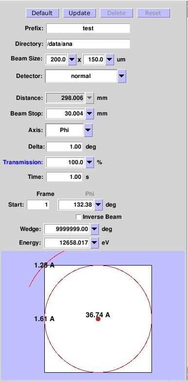
The Collect Tab (Figure 1) is used for collecting test images and complete monochromatic,
SAD and MAD data sets. Multiple run windows can be set up by creating
additional Run Tabs.
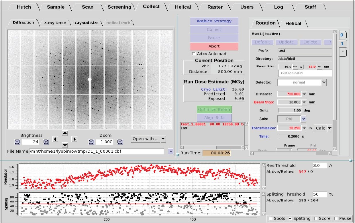
Figure 1. Collect Tab in BluIce
Data collection runs
- The Run tab 0 is the only run displayed when the collect
tab is first opened. It is a special run, dedicated for taking single test images in order to test
crystals and plan strategies for data collection. Only one image at
one time can be collected from this run, so it is not possible to
enter an end frame, although the drop down menu arrow next to the
phi value can be used to quickly set up image collection at 90
degrees away from the first image. A resolution
predictor widget displaying the resolution limits for the selected values of the detector, beamstop distance, and wavelength is available for this tab.
- To create additional data collection run, click on the
'*' tab below the '0' tab. Runs numbered 1
and above can be used to collect complete data sets at multiple energies.
Note: When you create a new "run", the contents
of the old run are automatically copied to the new run.
- There is a limit of 17 runs that can be defined. Once this
limit is reached, you must delete old runs in order to define new
ones. Data already collected in not affected by erasing the run.
Data collection parameters and commands
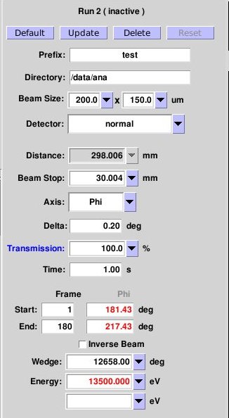
Figure 2. Data collection parameters and commands
Click on the links in Figure 2 for information on each parameter or input window.
- If you input data collection parameters by hand make sure that you do
not exceed the particular motor range. You can avoid this by
selecting values within the range defined by the drop-down
menu next to the input box. If you select a value outside this
range, the name of the parameter will be highlighted in
red. You will not be able to initiate the data collection.
- A motor or parameter value displayed in red indicates
that the motor is in a different position. The motor will move to
the position in red upon starting data collection.
- If you click on Default, the current values of distance, axis and energy will be selected
and displayed. In addition, prefix will be set to 'xtal',
directory to '/data/username'. The default detector mode, delta phi and
exposure time are different for each beamline.
- Click on Update if you wish to use the
current motor positions for the data collection. This is
useful if you have already set up the correct detector or
beamstop distance from the Hutch Tab. If you have mounted a
sample using the screening tab, update will also change the directory and image
prefix names to the ones defined in the screening tab. Similarly, if you have
done a MAD scan in the Scan Tab,
the optimal energies for a MAD experiment will be copied to
the run.
Important: Do NOT click on the Update button once
you have finished editing the collection run. This will
cancel all your edits.
- Use the Delete button to delete the run that you
are in. You cannot delete Run 0. Be careful when using this
command. Once a run is deleted, you cannot return to it.
- Use the Reset button to re-use a run. If you do
this you should change the image name or the destination
directory. If you do not change the names, Blu-Ice will create
a subdirectory called OVERWRITTEN_FILES where the old files
will be stored. This will protect the images from one
accidental overwrite.
- Another use of the Reset button is to edit data
collection parameters after stopping a started run (for
instance, to change the detector position). Note: if you
click "Collect" immediately after editing the run, data
collection will restart on the first image again. In order to
continue collection at the current frame, double-click on the
image name as explained in the Tips.
prefix
|
- Filename root or file prefix
|
directory
|
- Shows the directory in which the image will be
saved. Only directory paths starting with "/data" are allowed. When
you select this input box, a list of all the subdirectories in the
current directory will be displayed as a drop-down menu. You can
either select one of the existing directories, or type in a brand new
one.
|
beam size
|
- Beam size enables inputting various beam sizes for the
data collection. Please see the Adjusting Beam Size section
in the Sample_tab for more information.
|
detector
|
- Specific values for the detector depends
on the type of detectors. SSRL beamlines use so-called Pixel
Array Detectors: Dectris Pilatus 6M, Eiger 16M and Eiger2 XE 16M.
- The Pixel Array Detectors support shutterless data
collection in which the shutter does not close for image readout
except for the last image in a run or a wedge (if the run is
being divided in multiple wedges) or before collecting inverse
beam images. This works because the readout time is much shorter
than the time taken to expose each frame. See
information below about pausing the
run in shutterless collection mode.
|
distance
|
- Distance between detector and sample in millimeters; the
minimum distance is usually between 90 and 110 mm, depending
on the beamline.
|
beamstop
|
- Beamstop distance in millimeters.
|
attenuation/transmission
|
- Beam attenuation or transmission. Use to avoid overloaded spots when
collecting low or medium resolution data from strongly
diffracting crystals.
|
axis
|
- Phi is the only choice unless the beamline is
equipped with a Kappa diffractometer.
- When Kappa is not set to zero, you must collect using Omega.
- The rotation range of Omega is limited.
- On beamlines with a Kappa diffractometer Omega and Kappa are usually locked to prevent hardware
collisions, but can be unlocked if the experiment requires it: contact your support staff.
|
delta
|
- Oscillation length per image. For the Pilatus
and Eiger detectors a small delta (0.1 or 0.2 degrees) is
recommended because it improves the data statistics and the
detector readout time does not add up anything to the total collection time.
|
time
|
- Length of exposure time in seconds. Note that if you change the oscillation angle per
image, the exposure time should be changed by the same factor
to obtain an equivalent exposure per image.
|
start
|
- The number and phi value assigned to the first image.
|
end
|
- The number and phi value assigned to the final image.
|
inverse beam
|
- Rotates the crystal by 180 deg to collect the Friedel pairs for the input phi range.
- When inverse beam is used for a MAD experiment, the inverse beam
pass is collected before changing the energy.
|
wedge
|
- The phi rotation range that is collected
consecutively before rotating the crystal by 180 degrees (with inverse
beam) or changing energy (during Multi-wavelength experiments).
|
energy
|
- Energy or energies used for the experiment. As
you enter an energy value, an empty box appears for further energy
entries. The energy boxes can be auto-filled by clicking on the
Update button after doing a MAD scan. If you wish to skip one
or two of the selected energies, simple delete the value.
|
take microspec snapshot during run
|
- This option is available when enabled from the
Microspec Tab on beamlines equipped
with an in situ microspectrophotometer. When checked, the software
will automatically collect a UV spectrum after a number of frames
entered by the user. The number of frames defaults to the amount
specified by the wedge. The spectrum will always be collected at the
same orientation given by the phi angle selected by the user
(defaults to the data collection start). To calculate the optimal
phi to monitor the spectrum, please refer to the documentation
for the microspec tab.
|
Figure 3. Run parameters
Run Dose Estimate
- The Run Dose Estimate window in the Collect tab provides
information about X-ray absorption during data collection. The
window displays experimental Dose Limits based on the type of
experiment being performed, a calculated Predicted Dose based on
crystal parameters and data collection Run parameters, and an
estimate of the Exposed Dose as the experiment proceeds.
- In the figure, the Run Dose Estimate window (highlighted
in orange) shows the X-ray Dose Limit and displays a Predicted Dose
based on the sample crystal and the Run parameters. This example
displays a Predicted Dose estimate that exceeds the limit for data
collection at room temperature.
- The Dose Limit is defined as the dose which reduces the
sample to half it's diffracting power or the loss of useful
anomalous signal. The Dose Limit can be toggled by clicking on the
Limit (blue indicates a toggle). Current options include:
-
Cryo (30 MGy) - Experiments performed at ~100 K
-
Cryo Se-MAD (5 MGy) - Seleno-met Multi-wavelength Anomalous Diffraction experiments at ~100 K
-
Cryo S-SAD (3 MGy) - Sulfur Single-wavelength Anomalous Diffraction experiments at ~100 K
- Room Temp (0.38 MGy) - Room Temperature experiments
- The Predicted Dose (the Average Diffraction-weighted Dose)
is calculated using
RADDOSE3D. RADDOSE3D
is also a supported program that can be run independently from the
command line.
- The Exposed Dose is an estimate of how much dose the
crystal has absorbed once data collection is running or has finished.
The Predicted and Exposed Dose values will turn red to indicate a
warning that they exceed the Dose Limit (see Figure 4).
- NOTE: The Predicted and Exposed Doses only apply
to individual Runs since a translation of the sample to an
unexposed area is assumed between Runs. If the crystal is exposed
in the same position over multiple Runs, the total Predicted and
Exposed Dose will be the sum of the doses for each Run.
|
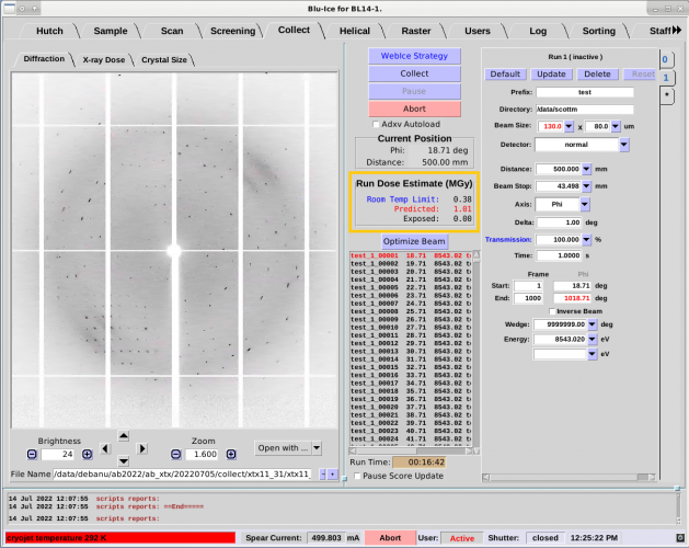
Figure 4. Collect Tab with Run Dose Estimate outlined in orange.
|
Default Crystal Parameters
- By default, a Predicted Dose will be calculated based on
a number of Default assumptions:
- The crystal is close to spherical or cubic in shape
- The crystal is larger than the beam size
- The protein is average in size
- No heavy metals
- Water solvent
- WARNING: If the above assumptions do not adequately
describe your crystal, the predicted dose will likely be
underestimated which can lead to an over-exposure of your sample.
In this case, use the X-ray Dose and the Crystal Size sub-tabs to
enter the appropriate sample information (see below).
X-ray Dose Sub-Tab
- Relevant information about the mounted sample will yield a
more accurate Run Dose Estimate. Sample parameters can be modified
in the X-ray Dose sub-tab (see Figure 5.).
- Unit Cell, Monomers and Residues. The unit cell can
be specified as well as the number of monomers in the unit cell and
the number of residues in each monomer. Alternatively, the molecular
weight of the monomer can be specified by clicking on the "Number of
Residues" parameter (blue indicates a toggle).
- Heavy Atoms. The type and number of heavy atoms in
each monomer can be specified. For example, four iron and six
selenium atoms in the monomer would be entered in the following
manner:
Fe 4 Se 6
- Solvent Content. The percentage of solvent content
can also be specified as well as the heavy atom concentrations in
the solvent. The type and concentration (mmol/l) of each heavy atom
type in the solvent can be specified. For example, concentrations of
100 mmol/l of P and 350 mmol/l of S and 50 mmol/l of Zn would be
entered in the following manner:
P 100 S 350 Zn 50.
NOTE: Atoms lighter than oxygen should not be included.
- Once the Dose Parameters in the X-ray Dose sub-tab have been
entered, click on "Apply" to update the Predicted Dose Estimate.
Values highlighted in red will be updated and a new Predicted Dose
will be calculated. Use the Cancel button before clicking Apply to
discard changes to the parameters.
- NOTE: The X-ray Dose sub-tab parameters apply to
the crystal that is currently mounted on the goniometer and
therefore these parameters apply to all Run tabs.
- At the bottom of the sub-tab, the crystal shape and size
are displayed as specified in the Crystal Size sub-tab. When a sample
is first mounted, the crystal shape and size default to a sphere
with radius about twice the size of the beam in
Blu-Ice.
The Crystal Size sub-tab can be used to redefine the crystal shape
and size for a more accurate estimate of the dose.
|
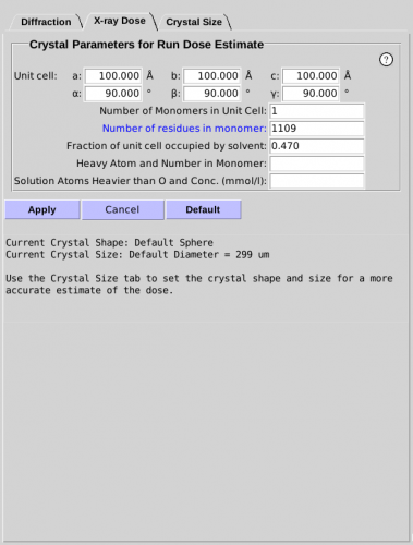
Figure 5. X-Ray Dose sub-tab.
|
Crystal Size Sub-Tab
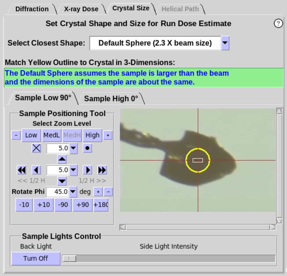
- The Crystal Size sub-tab (Figure 6, left)
provides an interactive tool to
define the shape and size of the mounted sample to give a more
accurate estimate of the absorbed dose. A yellow overlay
that defines the shape and size of the crystal is displayed on the
camera view of the sample.
- When a sample is first mounted, the shape defaults to
"Default Sphere(2.3 X beam size)". The default state assumes the crystal is
approximately the same size or larger than twice the beam size in
Blu-Ice. Thus, the diameter of the Default Sphere is
set to 2.3 times the current beam size in Blu-Ice
(i.e. the diameter is set to the Full Width of the Gaussian beam).
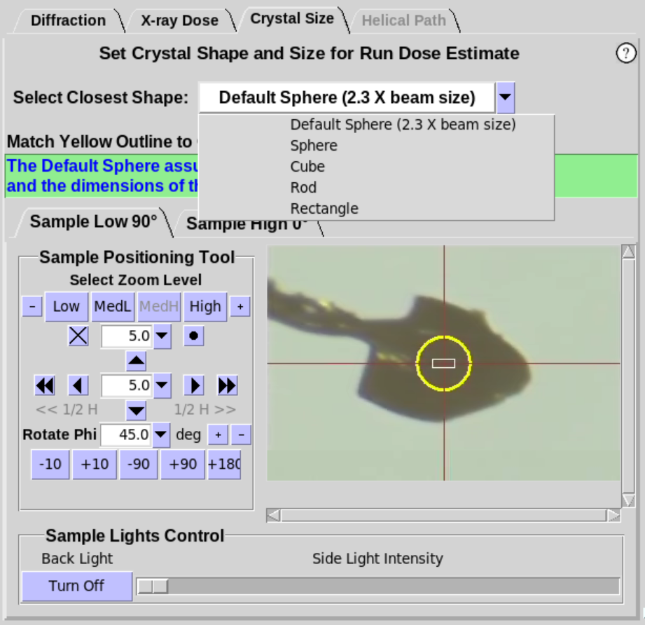
- Additional shapes with handles are available in the drop
down menu to better match the crystal shape and size for a more
accurate Dose Estimate (Figure 6, middle). Choose the shape that most closely
resembles the shape of the crystal. Resizing handles will appear on
the yellow overlay for Sphere and Rod (Figure 6, right). If the beamline
provides two camera views, either view can be used to adjust the
size of the overlay. Grab and move the handles with the mouse
(click and hold) to adjust the size of the circle/box to best fit
the crystal. Handles that are colored the same adjust the shape in
the same way. The crystal should be rotated about the Phi axis to
verify the crystal shape and size are adequately defined.
|
 |
 |
| 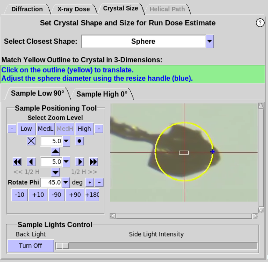 |
Figure 6. Crystal Size Sub-Tab.
- NOTE: The Predicted Dose is immediately updated
whenever the shape is changed or when the handles are used to change
the size of the crystal.
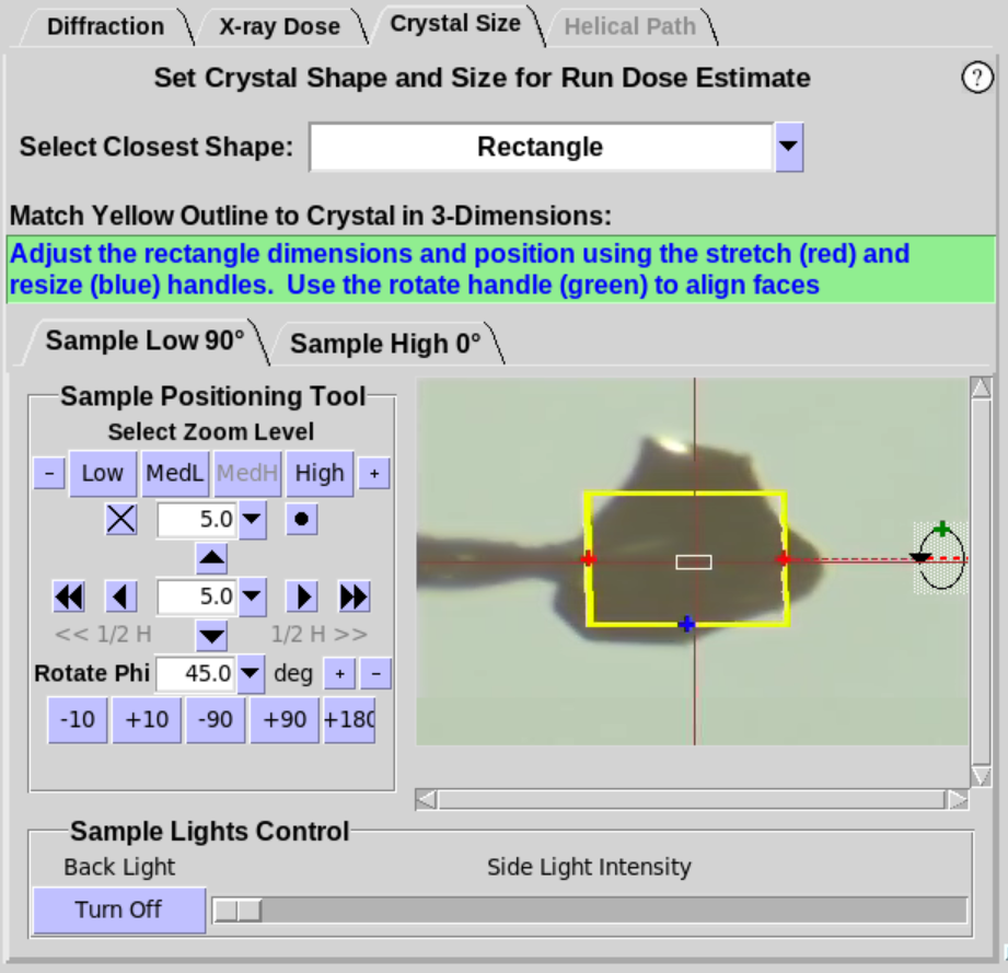
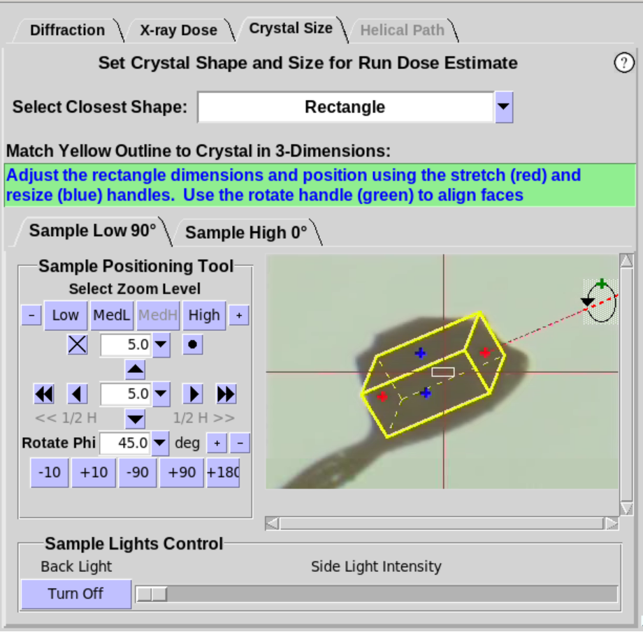
- When Cube or Rectangle are selected (Figure 7, left),
the crystal should be rotated about the Phi axis to align one of the
faces of the crystal approximately normal to the camera view. Once
the face of the crystal is aligned, two
handles will appear foradjusting the size of the yellow overlay to
match the face of the crystal (Figure 7, middle). Use the
+90 button to verify the yellow outline aligns with the crystal as
it is rotated. For the Rectangle shape,
an additional handle (green) will be available. Use the green handle to define the 3rd dimension of a
rectangular crystal (Figure 7, right).
- To use a different orientation of the crystal as the
initial "Face" of the Cube or Rectangle, rotate Phi to the new
location. The Cube or Rectangle
overlay can now be resized at this new Phi position.
- NOTE: If the crystal is not clearly visible, the
crystal can be rastered using low-dose X-rays to provide a
reasonable estimate of the crystal size. See the Rastering Tab
for more information on how to raster the crystal.
 |
 |
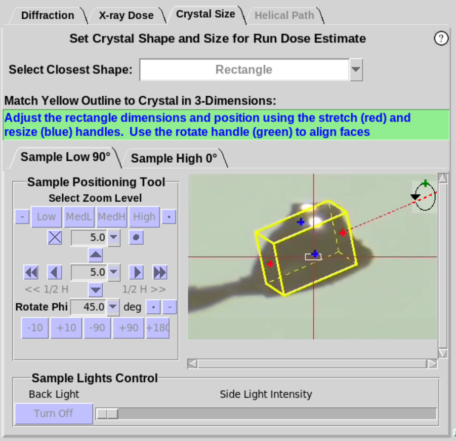 |
Figure 7. Crystal Size Sub-Tab, cont'd.
Data Collection Strategy
- Data collection strategies can be determined using the Strategy sub-tab in the Collect tab (Figure 8) and the results can be pulled into a particular Run using a new button called “Import Strategy” with the iMosflm Strategy icon (Figure 8, green arrow). The Strategy sub-tab runs the indexing and strategy options in iMosflm. As implemented, the Strategy calculation maximizes the completeness of the data set while minimizing the PHI rotation range; alternatively, it will determine a PHI range that will provide a specific multiplicity, if that target multiplicity has been specified by the user. If the "Anomalous" option is selected, a PHI range that maximizes the number of anomalous pairs or achieves the desired anomalous multiplicity (if specified) will be calculated.

Figure 8. Collect Tab with the Strategy Sub-tab.
- The image file text boxes in the Strategy sub-tab are populated with the filenames of the last few images collected in the Screening Tab or Run Tab 0. Select 2 compatible image files for indexing. A new option in Run Tab 0 makes it easier to collect two successive test images 90° apart. In Run Tab 0, check the “Auto-collect 2 images at Phi and Phi + 90°” checkbox (Figure 9, red arrow) for this feature to run automatically. Alternatively, one can select files using the "Browse" feature that opens a standard file dialog.

Figure 9. Run 0 tab with the checkbox to auto-collect two images for strategy.
- Once two files have been selected in the Strategy sub-tab, the "Run Strategy" button will be enabled. Click on the "Run Strategy" button and the resulting indexing and strategy parameters will be displayed in the bottom window. The output parameters include the image filenames and their corresponding phi angle ranges, the PHI angle difference between the images, resolution (estimated from the indexing solution), space group, unit cell, completeness, multiplicity, a starting and ending phi angle and phi Range for the proposed data collection strategy.
- Select “Completeness” and check the "Anomalous" checkbox to calculate a strategy that maximizes the completeness of unique symmetry-related reflection pairs for a minimum phi range. Selecting “Multiplicity” can be used with the anomalous flag to specify a target multiplicity of unique-symmetry related reflections.
- If the space group is known, enter it in the "Force Space Group" input box and click on the "Run Strategy" button; the user-defined space group will be used for indexing and the strategy calculation. If no space group is provided, the crystal system (i.e. Bravais lattice) will be determined ab initio, and the lowest-symmetry space group for that crystal system will be used for the strategy calculation. To calculate strategy at a specific resolution, enter the resolution into the "Force Resolution" input box and rerun strategy.
- Once the strategy calculation has completed successfully, the results can be transferred into a particular Run on the Collect Tab by clicking on the “Import Strategy” button (see figure above, green arrow). This action will only replace the starting and ending PHI values in the current Run Tab.
- Once the range has been set in the Run tab, check the Predicted Run Dose Estimate on the Collect Tab (Figure 8, red arrow), and adjust the exposure time accordingly. If the Predicted Dose is larger than the limit for the type of experiment selected, reduce the exposure time per image or consider using multiple crystals to achieve the desired completeness/multiplicity. If the Predicted Dose is much less than the experimental limit, consider increasing the exposure time per image to maximize data quality and resolution.
- Situations Where the Prediction Will Not Match the Processed Data:
- When a higher symmetry space group is determined during processing, there may be a mismatch between predicted and processed statistics because the strategy calculation assumes the lowest symmetry for the crystal system unless otherwise specified by the user. In these cases, more data would be collected than necessary; however, the completeness should be similar, and the multiplicity will be higher providing higher quality data (no data will be missing).
- When there is diffraction beyond the edge of the detector, there will be a mismatch because the resolution estimate used for strategy is truncated at the detector edge. If diffraction is observed close to or beyond the edge of the detector, a resolution beyond the edge can be entered into the Force Resolution box for the strategy calculation. This will give a more accurate prediction. However, data out to the corners beyond the edges of the detector will be heavily incomplete, therefore, one should reposition the detector to include all high-resolution data plus a ~0.3 Å margin.
Helical Data Collection
- The Helical Path Sub-Tab
(Figure 11) is located next to the Crystal Size Tab and allows collection
of oscillation data while the sample is translated along a predefined
path. On BL12-1 and BL12-2, the software collects oscillation
data in a continuous shutterless mode by setting the speed of the
translation for a constant exposure time. On BL14-1 and BL9-2, the
software collects an oscillation image then translates the sample to
a new position and collects the next image, etc.
- The best strategy to optimize diffraction resolution while
minimizing the effects of radiation damage is to expose the largest
possible volume of your crystal. When the crystal size is larger
than the largest beam size, use the Helical Data Collection option
to translate the entire crystal through the beam. First maximize the
vertical beam size to match the vertical size of the sample (if
possible) and then define a horizontal path to translate the crystal.
- The Path is defined by creating a graphic overlay on the
live video stream of the sample in the new Helical Path Sub-Tab (
described in detail below).
- Helical data collection is initiated and managed in the
same way as standard Rotation data collection which is described
extensively above in the
Collect Tab Manual.
- Any number of Frames can be specified. For BL12-1 and
BL12-2 where shutterless data collection is employed, the speed is
adjusted for an even exposure of the sample as it is translated and
rotation images are collected.
- The Default Button will set a default number of Frames for
the existing Path so that the exposure overlap is ~1/2 the horizontal
Gaussian beam size. If a larger dataset is desired, the number of
frames can be increased with a commensurate increase in the overlap
of the exposure area (typical strategy for collecting a full data set
from a single crystal). Likewise, exposures can be set farther apart
at the expense of collecting fewer Frames.
|
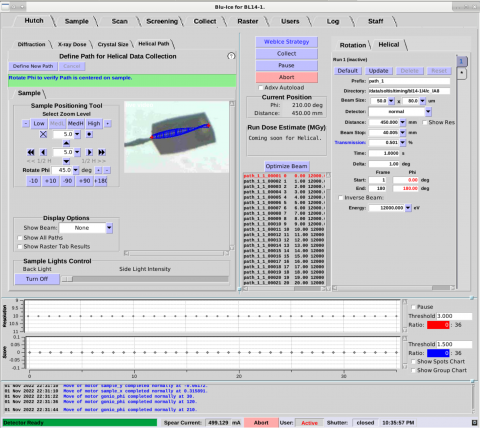 |
Figure 11. Helical Path sub-tab.
Helical Path Interface
- The Helical Path interface provides a graphical overlay on
the live camera view of the sample to set a path for helical data
collection (Figure 12). One Path can be defined for each Run and
up to 16 Runs (and thus 16 Paths) can be specified for each mounted
crystal (or multiple crystals on a mesh). Choose one end of your
sample for the starting point of the helical Path. Align the
starting point in the center of the beam (at phi and phi +90).
Press "Save Path Start". Choose the end of the helical path and
center it at the beam center. Press "Save Path End".
- NOTE: it is critical to rotate Phi 360 degrees to
verify the positioning of the Path is correct on the sample.
- NOTE: in crystal overlay displayed, the vertical
beam may appear to change in size because this image is a projection
at different Phi rotation values.
- To modify the Path, press "Define New Path".
- By default, only the associated Path is shown for the
selected Run as an overlay on the sample camera video. All Paths
can be shown by clicking on the "Show All Paths" checkbox. In
addition, results from the Raster Tab can be overlaid on the sample
by selecting the Show Raster Tab Results checkbox.
|
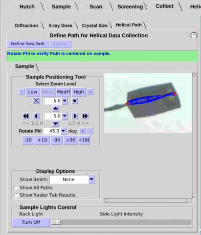 |
Figure 12. Helical Path interface.
Starting a Data Collection Run
- After setting all parameters to your desired values click Start to collect an image.
- The network status of your Blu-Ice Client must be Active to collect an image.
- If you have
created a few runs and start data collection from a previous "run", Blu-Ice will collect frames from the current run and the following runs (Note: Blu-Ice will not recollect frames from an already completed "run"). This allows users to collect multiple data sets (eg., low resolution pass, high resolution pass or different wavelengths) using different "run" windows.
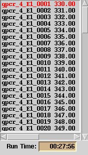
Run Time
- Run Time shows the time remaining for the data collection run. If new values of data collection parameters are entered in the
run definition, the run time is recalculated. During the run, the run time is updated after every image.
Data File Naming
- Each data file in your selected run sequence is named in
the following way: 'file prefix'_'run
number'_'energy number'_'image number'.img.
- For example, a file could be named data_2_E2_010.img. This image is in the
10th frame collected in Run 2 at the 2nd input energy.
- With only one energy level selected, the file would be name 'file prefix'_'run number'_'image number'.img.
Run Sequence
|
- The run sequence (Figure 13.) depends on the values for phi, wedge, energy or
inverse beam that you choose. The image collection
order will be displayed in the 'run sequence'
window. Below are examples of some possible run
sequences.
- Note: Once the current run is finished, the software will go on to
collect any unfinished runs (paused or inactive) following the current one.
|
One Energy, Inverse Beam Off,
Phi < Wedge Size
(simplest case)
test_1_001
test_1_002
test_1_003
(phi: 0-3 deg, wedge: 3 deg, 1 energy, inverse beam off)
|
Two or more Energies, Inverse Beam Off, Phi < Wedge Size
example:
test_1_E1_001
test_1_E1_002
test_1_E1_003
test_1_E2_001
test_1_E2_002
test_1_E2_003
(phi: 0-3 deg, wedge: 3 deg, 2 energies, inverse beam off)
|
Two or more Energies, Inverse Beam On, Phi < Wedge Size
example:
test_1_E1_001
test_1_E1_002
test_1_E1_003
test_1_E1_181
test_1_E1_182
test_1_E1_183
test_1_E2_001
test_1_E2_002
test_1_E2_003
test_1_E2_181
test_1_E2_182
test_1_E2_183
(phi: 0-3 deg, wedge: 3 deg, 2 energies, inverse beam on)
|
Two or more Energies, Inverse Beam On, Phi > Wedge Size
example:
test_1_E1_001
test_1_E1_002
test_1_E1_181
test_1_E1_182
test_1_E2_001
test_1_E2_002
test_1_E2_181
test_1_E2_182
test_1_E1_003
test_1_E1_183
test_1_E2_003
test_1_E2_183
(phi: 0 - 3 deg, wedge: 2 deg, 2 energies, inverse beam on) |
Figure 13. Run Sequence interface (above) with examples of run sequences (below).
Image display commands
Figure 14. Image display interface.
New images are displayed to the left of the collect tab as soon as
they are written to the users' area. Older images can be displayed and
inspected by launching the program ADXV.
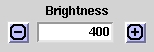
brightness
|
- The default image Brightness value is set to 400. Change this value for a desirable contrast between spots and background.
|
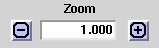
zoom
|
- Click on this to zoom in or out of the diffraction image.
|
move arrows
|
- Pans the image within the display box.
|
Alternative image viewers
|
- Allows the user to inspect and analyze diffraction images
with ADXV.
|
Select image
|
- Allows the user to select the previous and next images in
the run sequence with
the + and - buttons. To use this tool while data collection is
ongoing, click the Hold image check box.
|
Figure 15. Image display parameters.
Useful Tips
- Subdirectories are automatically created.
- The next image to be collected is colored red in the 'Run Sequence' box. You can jump to a different image if you double click on the desired image name.
- Pressing the "Pause" button stops the data
collection after completing the current frame, or, in the case
of shutterless data collection, after completion of the
current wedge.
- Pressing the "Abort" button immediately stops the data collection.
- Double-clicking on an image automatically starts ADXV.
Diffraction Quality Strip Chart
- The strip chart at the bottom of the Collect Tab displays
a few key data processing statistics in near real time (Figure 10).
The program
Interceptor is used to quickly process each
image as it is produced and the results are displayed in the strip
chart. Resolution, a Quality Score, the Number of
Spots, and the Likelihood of Spot Splitting are determined
for each image. The Score is primarily based on resolution, with
penalties and bonuses applied for number of ice rings, max intensity
between 15-4.5 Å, and spot elongation. Thresholds can be set to
indicate the number of images/frames that meet a particular
requirement (e.g. minimum resolution of 3.0 Angstrom) (in color) and
those that do not (in black). The chart can be paused by checking
the Pause checkbox. The Score, Spots, and
Splitcharts can be toggled on or off by selecting the
respective checkbox. The window can be resized vertically by
clicking on and dragging the square in the upper right corner of the
window.
- WARNING: These on-the-fly calculated statistics are
not as accurate as fully processed data. For a more accurate
assessment of your sample, please check the Automated Processing
directories for your particular dataset.
- Hovering over the chart area will produce a cross cursor
which can be used to select an area to zoom into (click and drag).
Multiple zooms can be used to see individual data points when
collecting images rapidly. Use Zoom Out in the context menu
(right click on the chart area) to zoom out to the previous zoom
area. Select View All to see all the data on the chart.
Hovering over a data point will bring up its value and image number.
Clicking on a data point will display the associated diffraction
image in the Diffraction Sub-Tab. To resume displaying images
as data are collected, uncheck the Hold Image checkbox in the
Diffraction Tab.
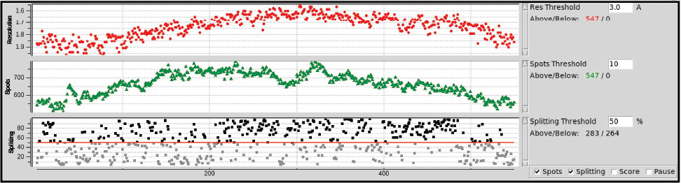 |
Figure 10. Diffration quality strip chart.
Automated Data Processing
- Once a run has completed with 10 or more images, the data are automatically processed providing quick feedback on the quality of the dataset. If a spreadsheet has been assigned to the cassette, the processing run information (and selected results) will be written into the Sample database. Once in the Sample database, the processing information will be displayed in the new Processing Tab. A complete description of automated processing and the new Processing Tab can be found here.
|