MicroSpec Tab
|
|
Introduction
This fully remote access capable microspectrophotometer enables the collection of UV-Vis absorption spectra. We expect that the most significant uses of this device will be for monitoring the photo-reduction of catalytic metal centers in enzyme active sites, but it is also useful for following enzymatic reactions or characterization of protein-ligand complexes that contain intrinsic chromophores.
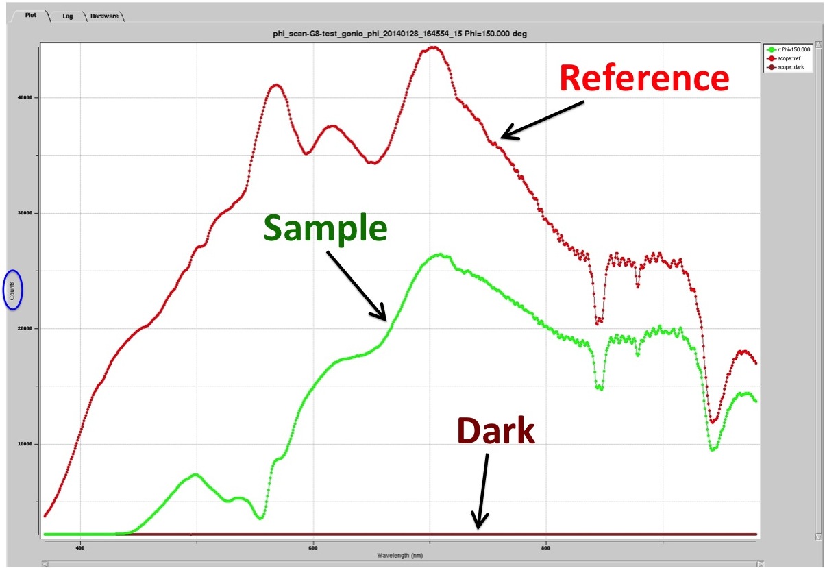
Absorbance spectrum is a measure of how much light a sample (e.g. crystal) absorbs, and it is calculated from the raw intensity counts data according to the following equation:
A = log10 [(R - D) / (S - D)]
where:
A = calculated sample absorbance at wavelength λ (AU)
S = sample transmitted intensity at wavelength λ (counts)
D = dark (background) intensity at wavelength λ (counts)
R = reference incident intensity at wavelength λ (counts)
In situ single crystal UV-Vis spectroscopy is a useful tool for identification and characterization of optical features of protein crystal samples, as well as for monitoring their sensitivity to the effects of the X-ray beam to aid in the design of the best strategy for X-ray data collection.
The software interface to setup the spectroscopic acquisition parameters and collect sample absorbance data is located in the Microspec Tab of the Blu-Ice.
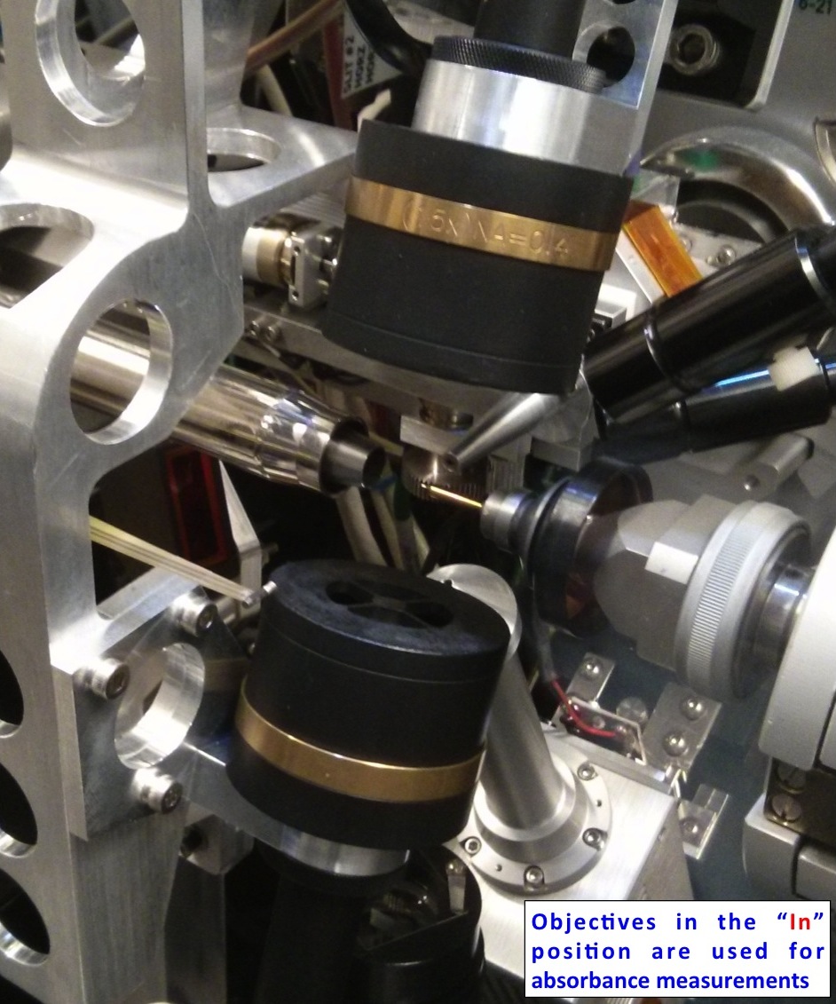
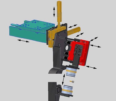
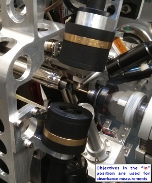
Note: The movement of objectives “in” (Figure 1A) and “out” (Figure 1B) is automated but with one exception – if you hit “Abort” button to stop a scan, then the objectives need to be removed manually by clicking “Remove” in the Hardware sub-tab of the Microspec Tab (see Table 1 for more details). In the sample measurement position, the objectives block the sample camera view (Figure 1A).
| 
|
| Figure 1A |
Figure 1B |
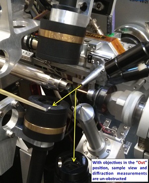
Figure 1 (Click to enlarge) Positions of microspec objectives for measuring A) absorbance (“in”) and B) diffraction (“out”).
Data Collection Procedure
- Select Lighting: Turn on the desired lamp(s) in the Light Control box on the Hardware Sub-Tab to allow for sufficient warm-up time to reach stable output.
- Select the appropriate acquisition settings: Values for time, averaging and boxcar should be selected with consideration from the Hardware Setup Sub-Tab (see Table 1 for more information).
- Align your sample: The microspec light spot is about 50 microns and centered in the X-ray beam position indicated by a white box in the camera view.
- Collect a new Dark and Reference:
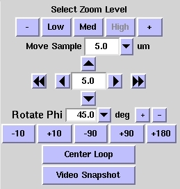
- Move your sample out of the light path: In High Zoom, click left double arrow 1-3 times – until sample is not in view. Depending on the size of your sample and where you center on it, it may take a few times to click. The actual distance translated with double arrow in High Zoom is small, so that sample stays in the cryostream but will not block the light path.
- Collect a new Dark and Reference: Go to the Microspec tab, the buttons to collect Dark and Reference are indicated by images of a light bulb. At the end, the microspec objectives will automatically move out from the sample position.
- Move your sample back into the light path: Go back to the sample camera view - in the same High Zoom, click right double arrow the same number of times as in Step 4a – this will bring your sample to the same centering position as it was in Step 3.
- Choose the optimum sample rotation: It is beneficial to use Phi-Rotation Mode to determine what orientation of your crystal (phi angle) results in a better quality spectrum. Go to the Microspec tab and use the Phi-Rotation Mode.
- Collect a Spectrum: Go to the Microspec tab to collect sample absorbance spectra using the desired data collection modes, which are described in sections below. (Single Spectrum, Phi-Rotation, X-ray Exposure, and Time modes)
- Collect X-ray data and (UV-)Visible spectra: After optimizing the crystal orientation (phi) in Phi-Rotation, stay in Microspec Tab and Enable Microspec Mode on Collect Tab, setup the spectroscopy parameters on the Hardware Sub-Tab. Then select optimized phi value and the frequency of spectra thru the wedge value.
- Your files are saved automatically in the directory as specified in the Scan Parameters box. File formats, content and data displaying options are described in the Spectroscopic Data Format Section.
The Spectrometer Hardware Setup Tab
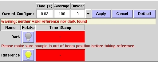
The Hardware sub-tab is used to configure the spectrometer and collect Dark and Reference spectra that are required for sample absorbance measurements.
The “Calculation Setup” box in the Hardware sub-tab allows user to configure the acquisition settings such as integration time, averages (number of accumulations) and boxcar (smoothing). Each integration time and boxcar settings will require its own Dark and Reference data, which are acquired using the same “Calculation Setup” box and the corresponding spectra are displayed below in the Graph sub-tab. The Hardware sub-tab is illustrated in Figure 2, and functions of various control features are summarized in Table 1.
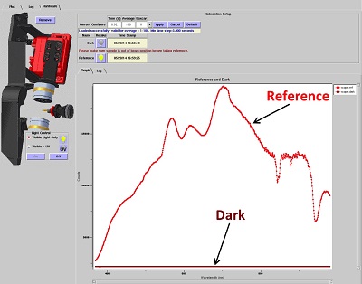
Figure 2 (Click to enlarge) Hardware sub-tab showing plot of Reference and Dark, “Calculation Setup” box, “Light Control” box, and “Remove” button.
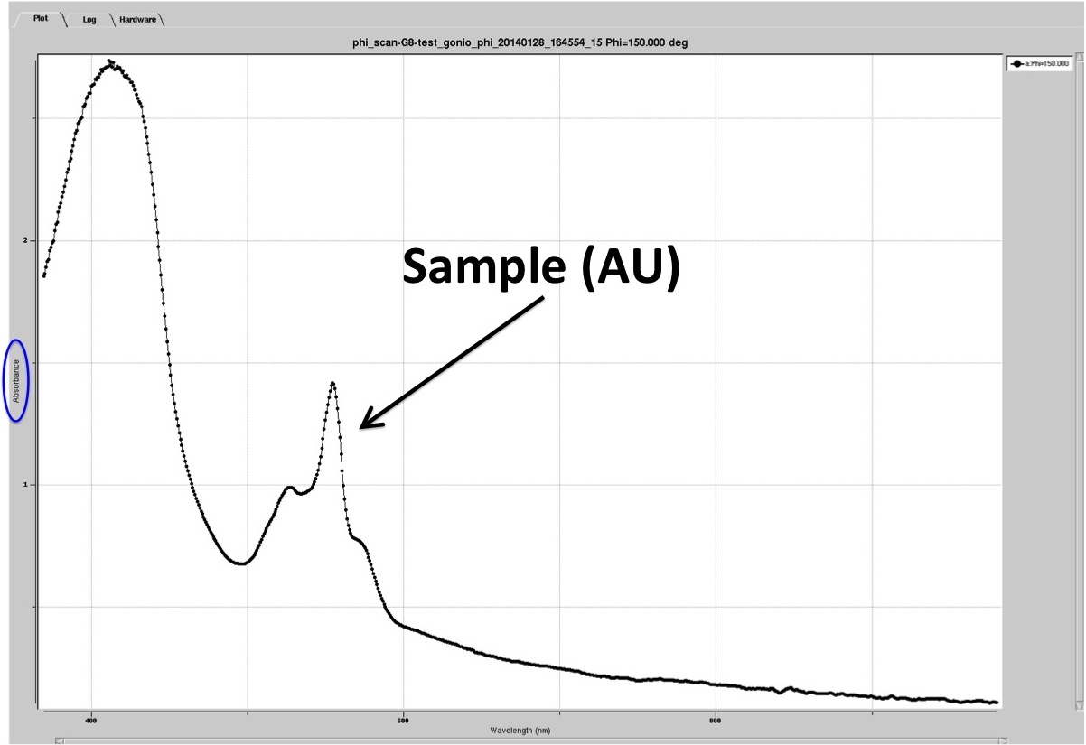
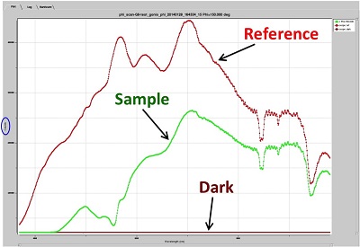
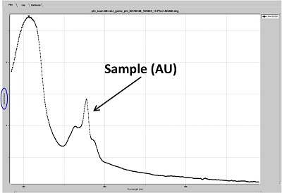
Sample spectra can be collected using several data collection modes that are available in the “Scan Mode” box, and can be setup in the “Scan Parameters” box in the main Microspec Tab (right side). These include Snapshot, Phi-Rotation, X-ray Exposure and Time modes, which are described in more detail in later sections. The sample absorbance spectra are calculated automatically (from the raw intensity spectra of Sample, Dark and Reference), and displayed in the Plot sub-tab of the Microspec Tab (e.g. Figure 3).
| 
|
| Figure 3A |
Figure 3B |
Figure 3 (Click to enlarge) Plot sub-tab showing spectroscopic data in units of A) raw intensity counts (Reference, Background and Sample), and B) calculated Sample absorbance.
| Table 1. Summary of Acquisition Setup Functions in the “Hardware” Sub-Tab.
|
| Control
|
Function
|
| Light Control
|
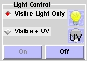
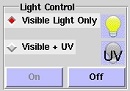
To acquire a visible spectrum (400 – 900 nm) select “visible light only”, which will turn on the halogen lamp in the lightsource. To collect spectral data in the UV-visible range (250 – 900 nm) select “visible + UV”, which will turn on both deuterium and halogen lamps in the lightsource.
The halogen lamp turns on immediately after the click, but there is some delay required for deuterium lamp to fully turn on. It is recommended to allow at least 15 min of warm-up time for optimal stabilization of the output.
To limit sample exposure, the lightsource shutter remains closed (when the lamps are turned on) and opens automatically only during data acquisition.
Note: long-term exposure to UV light may damage your sample.
|
| Calculation Setup
|
This box contains several configuration controls necessary to setup acquisition and processing of the spectral data.
|
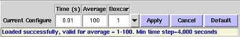
| Time
|
Specifies the integration time of the spectrometer, which is analogous to the shutter control of a camera.
For optimal performance, the raw intensity counts should stay below ~85% of the detector’s capability, which for QE65000 spectrometer is ~50,000 counts.
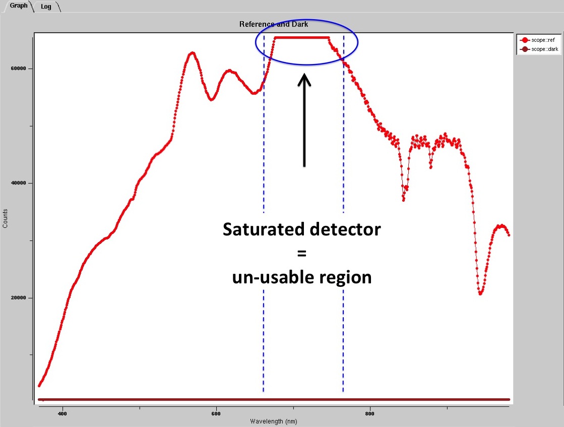
The minimal integration time is 0.01 seconds. To change a value, type in the desired number, hit “Apply”. If integration time is too high and detector is saturated – that region is unusable (eg. Figure 5).
|
| Average
|
Specifies the number of discrete spectral acquisitions that are accumulated prior to displaying the average spectrum. The higher the value, the better the signal-to-noise ratio (S/N). The S/N will improve by the square root of the number of scans averaged.
A value of 100 is set as a default for Dark and Reference, and if left unchanged by the user, will also be used to collect the Sample scan.
Lower average may be required for X-ray Exposure and Time Modes of data collection to reduce the total acquisition time per scan. The minimal time step (i.e. the frequency of acquisitions) is determined by hardware and is indicated in the message bar in the Calculation Setup box.
|
| Boxcar
|
Specifies the boxcar smoothing width, a filtering technique that averages across spectral data (i.e. a group of adjacent detector elements). For example, a value of 3 averages each data point with 3 points to its left and 3 points to its right (2N+1). A value of 0 indicates that no smoothing is performed on the spectrum.
CAUTION: The greater this value, the smoother the appearance of the data. However, if the value entered is too high, a loss in spectral resolution will result (over-smoothing). Better to collect un-smoothed data (i.e. boxcar=0), and then apply a smoothing algorithm later, if needed. In contrast, if data is collected with non-zero boxcar, it cannot be “un-smoothed” later to increase spectral resolution.
|
| Dark
|
Background light intensity detected by the spectrometer in the absence of incident light (i.e. lightsource). Given in units of raw counts, includes contributions from electric noise and stray light, and it is used in the calculation of the absorbance spectrum.
|
| Reference
|
Maximal incident light intensity, measured in the absence of sample in the light path (i.e. between illumination and collection objectives). Given in units of raw intensity counts and it is used in the calculation of the absorbance spectrum. The spectral profile is dependent on lamp(s) warm-up time and stabilization, optical fiber transmission properties and integration time.
|
| Graph sub-Tab
|
Displays a plot of Dark and Reference in counts vs wavelength
|
| Log sub-Tab
|
Displays values for Dark and Reference in a numerical format (columns of wavelength, counts (Dark), counts (Reference))
|
| REMOVE
|
Moves microspec objectives outside of the sample measurement position. Use this if you hit Abort during a scan, otherwise the positioning of the objectives “In” and “Out” is fully automated.
|
| Min time step
|
 How frequently consecutive scans can be collected is determined by the hardware, taking in to account integration time and number of averages. This may need to be adjusted for time-dependent data collection strategies such as Time Mode or X-ray Exposure Mode.
|
Dark and Reference
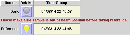
In order to proceed to collection of a Sample spectrum, a Reference and Dark spectra are required. If Dark and Reference files already exist for desired configuration (integration time and boxcar), the Time Stamp box will show when these were taken. Only use recently collected References and Darks. It is advisable to re-measure them frequently to account for fluctuations in lightsource output stability, among other factors.
Collecting a Dark
A Dark spectrum is a measure of background intensity (including electric noise and stray light), collected in the “dark” (i.e. in the absence of the incident light from the lightsource).
-
To collect a “Dark”, click on the light bulb button to the right of the word "Dark". The time stamp should update to reflect that a new Dark file was successfully saved.
The graph below the “Calculation Setup” box will show a spectrum, which should consist of very low counts across all wavelengths (e.g. brown spectrum in Figure 2 or Figure 3A). The same window has a log tab that will display the actual data points in the column format (wavelength and raw counts).
Collecting a Reference
A Reference spectrum is the measure of the maximal incident intensity from the light source, in the absence of a sample in-between the illumination and collection objectives.
To achieve a consistent Reference spectrum, it is advisable to let the selected lamp(s) in the lightsource to warm-up for at least 15 minutes to reach a stable light output.
-
 Use the “Light Control” box to select a region of the optical spectrum you would like to collect data on. To acquire a visible spectrum (400 – 900 nm) select “visible light only”, which will turn on the halogen lamp in the lightsource. To collect spectral data in the UV-visible range (250 – 900 nm) select “visible + UV”, which will turn on both deuterium and halogen lamps in the lightsource. Although the lamps will turn on, the lightsource shutter will remain closed until spectral data acquisition starts.
- Make sure that the sample is completely out of the light path, so that accurate Reference spectrum can be collected. To do this either dismount your sample or temporarily translate your centered sample out of the light path (see Data Collection Procedure).
- To collect the Reference scan, click on the light bulb image next to the word “Reference” in the Calculation Setup box.
The microspec objectives will automatically move in to the sample position (e.g. as shown in Figure 1A), the lightsource shutter will open to acquire the Reference spectrum, and the objectives will move back out (e.g. as in Figure 1B). The time stamp should update to reflect that a new Reference file was successfully saved. The graph below should show a spectrum similar to the red spectra in Figure 2 (Visible) or Figure 4 (UV + Visible). The same window has a log tab that will display the actual data points in the column format (wavelength and raw counts).
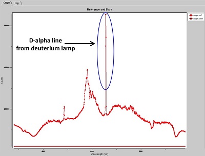
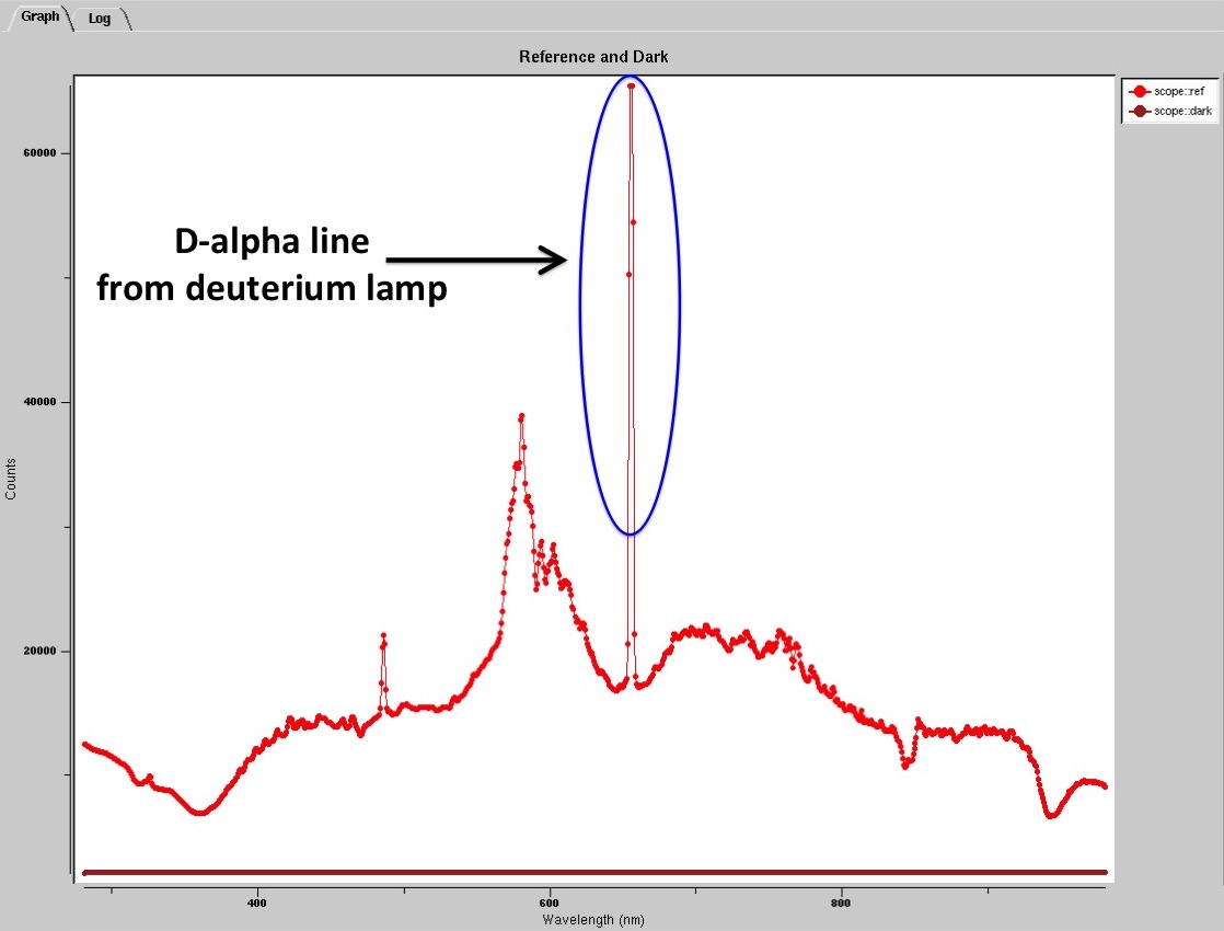
Figure 4 (Click to enlarge) Example of Dark and Reference spectra (raw intensity counts) collected for UV + Visible spectral range.
Check the Reference spectrum to make sure that there is no saturation at any point. All points must be below 65,000 counts (Y-axis) and, ideally, the majority should be under 50,000 counts. Short integration times will ensure that the detector will not saturate. Integration times of 0.01 – 0.02 seconds for UV + Visible range, and 0.02 – 0.03 seconds for Visible range are recommended.
An example of saturated and thus un-usable Reference spectrum is illustrated in Figure 5, where a significant portion of the spectrum exceeds the allowed detector limit, and cannot be used for accurate calculation of sample absorbance. In this case, the integration time must be reduced to bring the entire intensity profile within detector limits, and Reference re-collected (e.g. Figure 2).
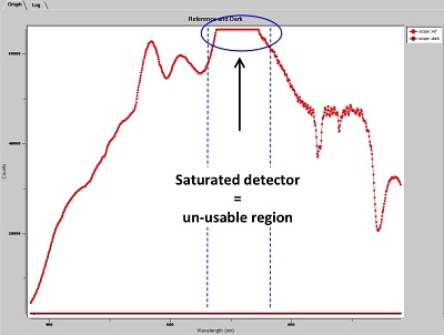
Figure 5 (Click to enlarge) Example of saturated and thus un-usable Reference spectrum. Re-collection with shorter integration time is required.
Exception: The reference spectrum collected for “UV + visible” range reveals a sharp and very intense peak observed around 655 nm (Figure 4). This is a D-alpha line, which is a feature of all deuterium-tungsten lamps. Correcting for this D-alpha line is difficult without compromising the intensity of the entire spectral range. If the boxcar values are small or zero, this line is narrow and only a few points are saturating and can be ignored in the absorbance spectrum. However, at high boxcar values this line is “smoothed” and broadened, which creates much wider and still very intense peak and, as consequence, more of an artifact in the absorbance spectrum.
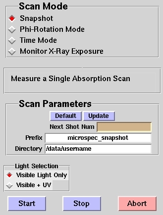
Snapshot (Single Spectrum) Mode
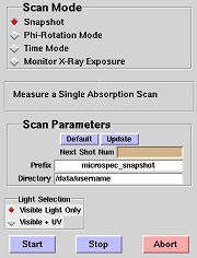
In this mode a single absorbance spectrum is collected on a centered crystal position and orientation.
- Use the Snapshot selection under Scan Mode in the MicroSpec Tab.
- In the Scan Parameters box, enter file prefix and directory as desired.
- Make sure the light (Visible or UV + Visible) is turned on and selected lamp(s) are allowed to warm up, Dark and Reference scans have been taken, and sample is centered in desired position.
- Click Start to collect a single spectrum.
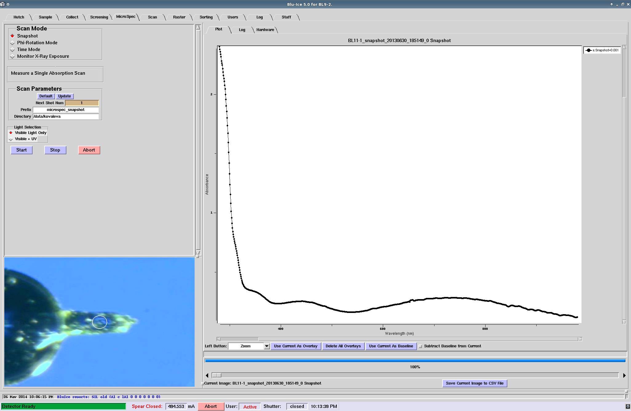
What happens - First, a camera snapshot of your sample is taken (at the phi specified). Then microspec objectives will automatically move to the sample position and the light source shutter will open to collect a sample spectrum. Both the camera snapshot of your crystal and a collected absorbance spectrum (Figure 6) are displayed in the Microspec Tab.
Note: for routine data collection, it is beneficial to use Phi-Rotation Mode first, to determine what orientation of your crystal (phi angle) results in a better quality spectrum. Then a Snapshot (Single Spectrum) Mode could be used at the best orientation to, for example, collect a spectrum with higher accumulation (higher average parameter, longer total acquisition time).

Figure 6 (Click to enlarge) View of the Microspec Tab in a “Snapshot” mode, illustrating a single absorbance spectrum and a corresponding camera snapshot of a crystal.
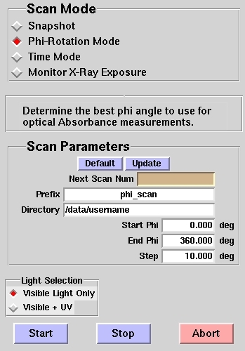
Phi-Rotation Mode
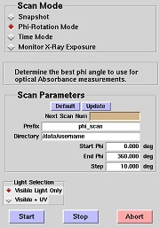
This automated feature allows to determine the best orientation of a crystal for absorbance measurements. Factors such as internal reflections from the frozen mother liquor, ice, cracks in the crystal, or the nylon loop can introduce spectral artifacts and thus diminish the quality of the crystal sample spectrum.
- Use the Phi-Rotation selection under Scan Mode in the MicroSpec Tab.
- In the Scan Parameters box, define the phi rotation range and step size. A good start is to scan from 0 – 360 degrees in 10 degree steps (i.e. Start Phi = 0; End Phi = 360; Step = 10)
- Also in the Scan Parameters box, enter file prefix and directory as desired.
- Make sure the light (Visible or UV + Visible) is turned on and selected lamp(s) are allowed to warm up, Dark and Reference scans have been taken, and sample is centered in desired position.
- Click Start to collect a series of spectra as a function of Phi angle.
What happens - First, a series of camera snapshots of your sample are taken at each phi value for which spectra are to be collected. Then microspec objectives will automatically move to the sample position and the lightsource shutter will open to collect sample spectra as a function of phi rotation (in the range and step size specified). For each phi value, both the camera snapshot of your crystal and a collected absorbance spectrum are displayed in the Plot window of the Microspec Tab.
The Progress Bar below the plot will tell you the progress of the scan series. The Slider Bar is useful to scroll quickly through the scans and determine the optimal orientation (Phi) of your crystal that gives the best quality spectrum. (Figure 7).
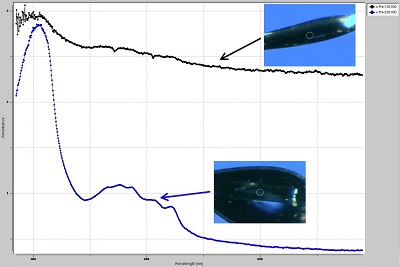
Figure 7 (Click to enlarge) Comparison of absorbance spectra collected at the optimal crystal orientation and that which includes interference from the nylon loop.
Note: If you click abort to stop the scan, you must click “Remove” in the Hardware Tab to remove the microspec objectives from the sample position (and X-ray beam path).
X-ray Exposure Mode
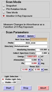
This mode is designed to monitor changes in the optical absorbance features as a function of X-ray exposure. This is a useful strategy to evaluate radiation-sensitivity of the chromophoric species (e.g. catalytic metals, ligands, co-factors, etc) using a test crystal to evaluate the X-ray dose and design X-ray data collection strategy.
- To take full advantage of this mode, it is best to first determine the optimal phi angle using the Phi-Rotation Mode before exposing your test crystal to the X-ray beam. Once the orientation of the crystal that gives the best quality spectrum is determined, move Phi to that angle value.
- Select Monitor X-ray Exposure Mode under Scan Mode.
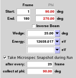
- In the Scan Parameters box, define the parameters for X-ray exposure (X-ray beam energy, attenuation, and beam size). The beam energy will be carried over from whatever value was last used. If a new value is entered, beam optimization will automatically precede spectral data acquisition.
- In the Scan Parameters box, define the parameters for spectral data acquisition series (monitoring duration and scan frequency). Note: the shortest time between each spectral scan is pre-determined by the hardware, including your set value for accumulations to average in the Calculation Setup box of the Hardware Tab (see Min Time Step value indicator in Figure 2 and Table 1).
- In the Scan Parameters box, check to make sure that the Phi angle is set to that determined from the Phi-Rotation Mode scan.
- Also in the Scan Parameters box, enter file prefix and directory as desired.
- Make sure the light (Visible or UV + Visible) is turned on and selected lamp(s) are allowed to warm up, Dark and Reference scans have been taken, and sample is centered in desired position.
- Click Start to collect a series of spectra as a function of X-ray exposure.
What happens - First, a camera snapshot of your sample is taken at a Phi value specified. If energy differs from that set in the Hutch Tab, beam optimization is performed. Then microspec objectives will automatically move to the sample position and the lightsource shutter and X-ray shutter will open in accordance with specified parameters.
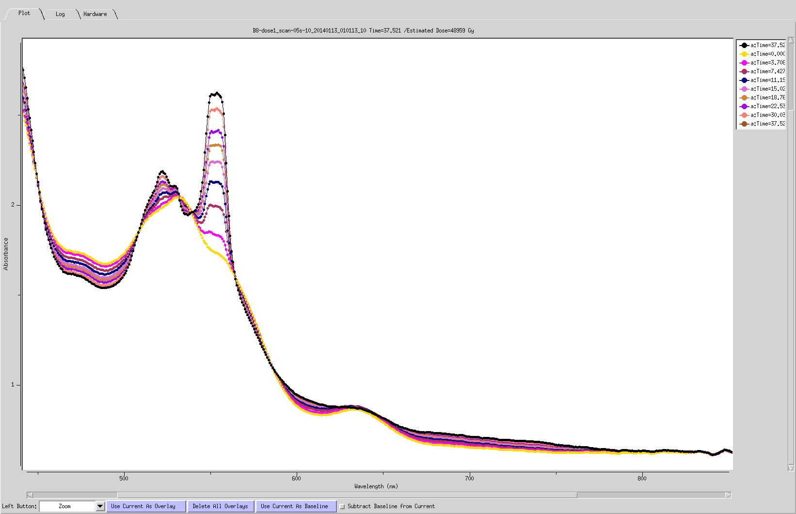
The Progress Bar below the plot will tell you the progress of the scan series. The Slider Bar is useful to scroll quickly through the scans to examine the dose-dependent effects on the optical features of your sample (Figure 8) For easy comparison of multiple absorbance scans in the Plot window, “Use Current as Overlay” button to save selected scans in the display (see Display and Scan Analysis Functions for more detail).
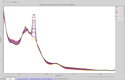
Figure 8 (Click to enlarge) Example of changes in the optical absorbance as a function of X-ray exposure.
Note: If you click abort to stop the scan, you must click “Remove” in The Hardware Tab to remove the microspec objectives from the sample position (and X-ray beam path).
The displayed dose values are estimates based on an ion-chamber reading that is calibrated on a biweekly basis.
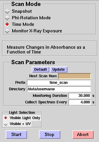
Time Mode
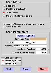
Time Mode enables you to measure absorbance at a fixed orientation of the crystal as a function of time (i.e. kinetic series). This is useful for triggered reactions. To set up a custom experiment, please contact your user support for help.
- To take full advantage of this mode, it is best to first determine the optimal phi angle using the Phi-Rotation Mode before reaction initiation. Once the orientation of the crystal that gives the best quality spectrum is determined, move Phi to that angle value (using Hutch Tab).
- Select Time Mode under Scan Mode.
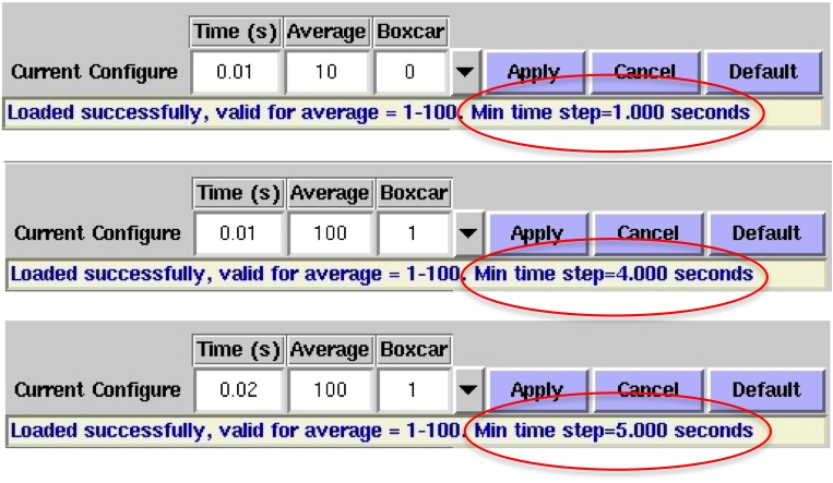
- In the Scan Parameters box, define the parameters for spectral data acquisition series (monitoring duration and scan frequency). Note: the shortest time between each spectral scan is pre-determined by the hardware, including your set value for accumulations to average in the Calculation Setup box of the Hardware Tab (see examples of Min Time Step value indicator in Figure 9.
- Also in the Scan Parameters box, enter file prefix and directory as desired.
- Make sure the light (Visible or UV + Visible) is turned on and selected lamp(s) are allowed to warm up, Dark and Reference scans have been taken, and sample is centered in desired position.
- Initiate the reaction (custom setup), and click Start to collect a kinetic series of spectra following external reaction triggering within the crystal.

Figure 9 (Click to enlarge) Combined effects of the parameter values for integration time and averaging on the Min Time Step required between consecutive spectral acquisitions.
What happens - First, a camera snapshot of your sample is taken at a phi value specified. Then microspec objectives will automatically move to the sample position and the lightsource shutter will open to collect sample spectra in accordance with specified parameters (range and step size) and the type of custom reaction trigger (contact user support for arrangements).
A series of absorbance spectra collected at different timepoints post-triggering will be displayed in the Plot window. The Progress Bar below the plot will tell you the progress of the scan series. The Slider Bar is useful to scroll quickly through the scans to examine the time-dependent changes in the optical absorbance features of your sample. For easy comparison of multiple absorbance scans in the Plot window, “Use Current as Overlay” button to save selected scans in the display (see Display and Scan Analysis Functions for more detail).
Note:If you click abort to stop the scan, you must click “Remove” in The Hardware Tab to remove the microspec objectives from the sample position (and X-ray beam path).
Interleaving Diffraction and Absorption Spectra Measurements
It is possible to combine collection of X-ray diffraction data and UV-Visible
spectra at predetermined (optimal) orientation of the crystal on the
goniometer by checking the Enable Microspec Mode on Collect
Tab button (see Figure
10). The optimal crystal orientation (phi angle) to collect the
UV spectra should be determined as described above in
the Phi-Rotation
Mode. The phi angle and the desired frequency of UV data
collection during X-ray data collection are then specified in
the Collect Tab. Please note
that increasing the frequency of UV spectra during data collection
will increase substantially the total time of the experiment.

(A) |
(B) |
Figure10 (Click to enlarge): (A) Microspec Tab a checkbox enables the option for combined X-ray diffraction and visible absorption spectroscopy measurements in the Collect tab. The Hardware sub-tab may be used to setup the spectroscopy collection parameters (such as UV-Visible or in Visible mode). (B) Collect Tab a setup box enables control of the frequency of absorption spectra collection and the desired orientation of the crystal during the collection (phi).
What happens - First, a camera snapshot of your sample is
taken at a Phi value specified in the Collect
Tab. Then, the microspec objectives will automatically move to
the sample position and the lightsource shutter and collect the
initial (UV-)Visible spectrum. It will be helpful to select Use
Current as Overlay to keep the unexposed crystal spectrum
displayed. Then, the X-ray diffraction data collection will start
until all the frames in the current wedge are recorded. Then, the
goniometer will return to the specified phi value and a UV-Visible
spectrum will be collected. This will continue iuntill all the
images in the data collection run have been collected. If the Use
Current as Overlay button is pressed in the Microspec Tab
after each spectrum is collected, a Graph similar to Figure 8 should be produced.
Processing: - Process the x-ray data as usual. For plotting
and displaying the collected spectroscopy data, you can load each
individual spectrum in BluIce and save the file into
a CVS file. If you need to process the spectra after your beamtime,
contact support staff to obtain access to the SIM9-2 simulator. For
more details, read the next chapter Spectroscopic Data Formats.
Spectroscopic Data Formats
Saved Data Files
For each spectroscopic dataset, a directory is automatically created in the location specified in the “Scan Parameters” box with the name given in the “prefix” field and the run number (e.g. data/username/prefix_1/). For all of the data collection modes, these directories will contain the following data files:
- CSV file – a master file that contains data acquisition parameters in the header, and datasets in the column format. These include wavelength, raw intensity counts for Dark, Reference and Sample scans, as well as calculated absorbance values. Use this file to import in to spreadsheet programs such as Excel.
- JPG files – camera snapshots of your sample at each phi value taken in the beginning of the data collection (single for Snapshot, X-ray Exposure and Time Modes; multiple for Phi-Rotation Mode).
- YAML files – “human-readable-data-serialization” format files.
- Master file contains information about entire multi-scan dataset specific for each Mode of data collection. Use this file to load into Blu-Ice for viewing.
- Individual files (_0, _1, _2, _etc) specific for each scan in the dataset.
Example of naming convention for folders and data files created for Phi-Rotation Mode:
/data/username/prefix_1/prefix_gonio_phi_date_time.csv
/data/username/prefix_1/prefix_gonio_phi_date_time_0.jpg
/data/username/prefix_1/prefix_gonio_phi_date_time_1.jpg
/data/username/prefix_1/prefix_gonio_phi_date_time_etc.jpg
/data/username/prefix_1/prefix_gonio_phi_date_time.yaml
/data/username/prefix_1/prefix_gonio_phi_date_time_0.yaml
/data/username/prefix_1/prefix_gonio_phi_date_time_1.yaml
/data/username/prefix_1/prefix_gonio_phi_date_time_etc.yaml
Display and Scan Analysis Functions
Right-Click on the Plot area functions:
- “Show Grid” – displays a grid in the plot area (on/off)
- “Show Zero” – changes autoscale of the Y-axis to start at 0 (on/off)
- “Zoom Out” – reduces zoom in increments
- “View All” – maximizes entire plot
- “Print” – allows to save the Plot window screenshot (PDF format) in the user specified directory
- “Load Scan” – allows to select a file to load from the selected directories
- “Show Scope” – displays current spectra collected (on/off)
- other spectra – displays data files loaded and used as overlays (on/off)
Right-Click on the Y-Axis functions:
- “Raw” – display sample scan in units of raw intensity counts
- “Counts” – display Dark, Reference and Sample scans in units of raw intensity counts
- “Reference” – display Reference in units of raw intensity counts
- “Dark” – display Dark in units of raw intensity counts
- “Absorbance” – display Sample scan in units of calculated absorbance (default)
- “Calculation” – display Sample scan in units of calculated absorbance and transmittance
- “Transmittance” – display Sample scan in units of calculated transmittance
Right-Click on the absorbance scan functions:
- “Phi angle and Scan name” – displays the value of Phi and filename for the scan or saved overlay
- “Set color” – choose color for the displayed absorbance scan
- “Set line thickness” – choose line thickness for the displayed absorbance scan
- “Set symbol” – choose symbols for the displayed absorbance scan
- “Set symbol size” – choose symbol size for the displayed absorbance scan
- “Delete scan” – remove this absorbance scan from display
Left Button pull down menu:
- “Zoom” – define area to zoom in (default)
- “Marker 1” – creates crosshair (default color red). Left-click on the plot to create; right-click on the crosshair to hide or to change color or line thickness.
- “Marker 2” – creates crosshair (default color green). Left-click on the plot to create; right-click on the crosshair to hide or to change color or line thickness.
- “% Marker” – creates crosshair (default color brown). Left-click on the plot to create; right-click on the crosshair to hide or to change color or line thickness.
Functions underneath the plot:
- “Progress and Slider Bar” – allows to scroll thru the series of scans collected in Phi-Rotation, X-ray Exposure and Time Modes (single scan displayed).
- “Use Current as Overlay” – saves the selected scan in the display (useful for comparisons of multiple scans)
- “Delete All Overlays” – removes all selected overlay scans, leaving default active scan displayed.
- “Use Current as Baseline” – selects a scan to be used as a baseline for baseline subtraction
- “Subtract Baseline from Current” – subtracts scan selected as a baseline from the current scan
- “Save Current as CSV” – saves current scan in CSV format.
- “Move to Phi” – used in combination with the scroll bar, displays the Phi angle of the currently displayed scan from the Phi-Rotation scan. If clicked, the Phi is moved to the indicated value
Viewing Saved Spectra in Blu-Ice
To view saved spectra files in Blu-Ice you need to load a master yaml file. In the Plot sub-tab of the Microspec Tab, right-click on the plot area to see a menu of functions and select “Load Scan”.
Note: you need to select an appropriate “Scan Mode” to load either single (Snapshot) or multi-scan dataset (Phi-Rotation, X-ray Exposure, Time).
- In Snapshot Mode – only can load a Snapshot scan (with camera snapshot displayed)
- In Phi-Rotation Mode
- can load Phi-Rotation dataset (with absorbance scans and camera snapshots displayed)
- Snapshot or X-ray Exposure datasets, if loaded, will display absorbance scans but not camera snapshots of the crystal
- In X-ray Exposure Mode
- can load X-ray Exposure dataset (with absorbance scans and camera snapshots displayed)
- Snapshot or Phi-Rotation datasets, if loaded, will display absorbance scans but not camera snapshots of the crystal
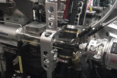
Hardware Description
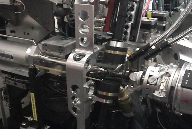
This new UV-Vis microspectrometer is motorized and its operation is fully automated. A 5-axis pico-motor stage is used to align the microspec objectives to each other. Three larger stages are used to align the pair of objectives to the sample position. By default, ~ 50 micron light spot at the sample is used. If necessary, your user support can change the fiber to produce a 5 micron light spot (advanced notice required, Visible range only). The system uses a Hamamatsu light source with deuterium and halogen lamps, UV solarization-resistant optical fibers, reflective Newport Schwardchild objectives, and an Ocean Optics QE65000 Spectrum Analyzer.
(Click to enlarge)
When not in use, the microspec is positioned away from the sample, in a position that would not interfere with standard functions such as sample mounting, alignment or X-ray diffraction data collection. For spectroscopic measurements, the microspec objectives will automatically move in to the sample measurement position (Figure 1A). At the end of the measurement, the microspec objectives will automatically move back out (Figure 1B).
Note: The movement of objectives “in” and “out” is automated but with one exception – if you hit “Abort” button to stop a scan, then the objectives need to be removed manually by clicking “Remove” in the Hardware sub-tab of the Microspec Tab (Figure 2, Table 1). In the sample measurement position, the objectives block the sample camera view (e.g. Figure 1A).
|