Processing Tab

Table of Contents


Overview

Once a data collection Run has completed with 10 or more images, the data are automatically processed using ICEflow - an SSRL automated pipeline that runs several 3rd party data processing applications that provide quick feedback on the quality of each data set.

Data processing run information and selected results are written to the Sample Database.

Once the run information appears in the database, selected information is diplayed in the Processing Tab.

Currently, autoPROC is used to run procesing for two different reolution cutoffs for each dataset. If autoPROC detects an anomalous signal it will spawn two new jobs with anomalous flags to optimize anomalous data processing.

If the Processing Tab is not displaying processing information:

  • Make sure a spreadsheet has been assigned to the cassette in the Screening Tab (which is currently required for writing to the Sample Database). A default spreadsheet can be created and assigned to the cassette.
  • If you have assigned the correct spreadsheet to your cassette in the Screening Tab and you still cannot see processing information, contact beamline support staff.

If a group does not want auto-processing results written to the Sample Database, they can opt out by checking the appropriate checkbox on the SSRL SMB Unix account request form (applies upon submittal) or by contacting their support staff. If a group opts out, no results will be recorded in our database or displayed in the Processing Tab, however auto-processing will still be carried out and the results can be found in the auto-processing directories (described below.).
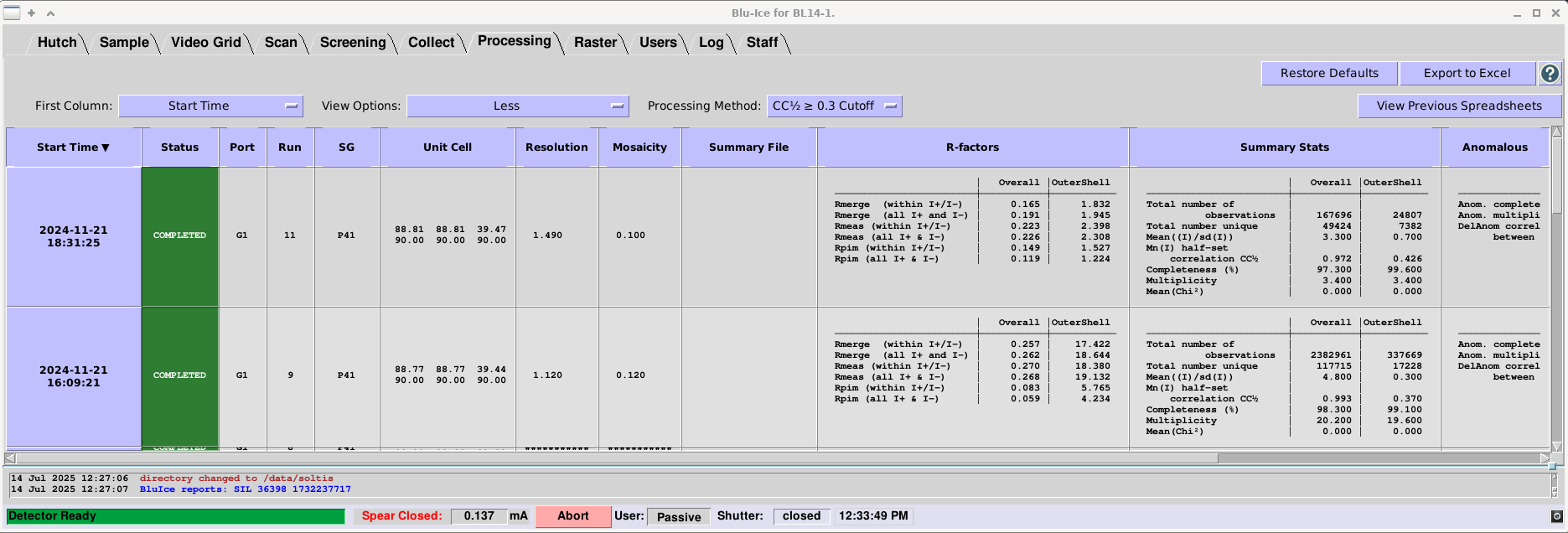
Processing Tab Overview


Layout and Navigation

Each row displays information and selected results for each data processing run; the table can be quickly traversed using scroll bars or arrow keys. The widths of the table columns can be changed by hovering the mouse pointer near the side of the column. When the pointer turns into a cross, click and drag the side of the column to the desired width.

Display Options

First Column

This drop down menu allows the user to select the first column which is fixed in place (default: Start Time) - the column stays in view when the table is scrolled horizontally.
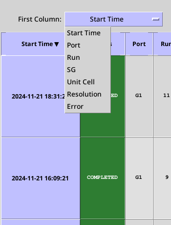
Figure: Processing spreadsheet sorting by column.

View Options

This drop-down menu can be used to select from several displays: Minimum, Less, More, or All:

  • Minimum - a bare-bones configuration showing essential information:
    • Start Time
    • Status
    • Port
    • Run
    • SG
    • Unit Cell
    • Resolution
    • [Resolution cutoff]
    • Summary file
    • Error
  • Less - a configuration showing additional summary statistics:
    • Mosaicity
    • Anisotropy
    • R-factors
    • Summary Stats
    • Anomalous Signal
  • More - a comprehensive list that also includes:
    • Crystal ID
    • Protein
    • Filename
    • Image Directory
    • Processing Directory
    • 3rd Party Pipeline
    • 3rd Party Pipeline Version
  • All - adds information for staff troubleshooting:
    • Run Time
    • Sample ID
    • Spreadsheet ID
    • Job ID
    • Slurm Job ID
    • Slurm Job Name
    • Slurm Partition
    • Hostname

Processing Method

This drop-down menu can be used to view the results for different resolution cutoffs (i.e. CC12, I/σ(I), etc.).

Table Sorting

By default, the table is sorted on Start Time (when the job was submitted to the queue) and the column is sorted with the last submission on top. However, any column can be used as the primary sorting column by simply clicking on the column title. By clicking on the arrow in the column heading, sorting can be reversed.

Two-column sorting is possible by clicking on a second column title anywhere in the spreadsheet which will then become the primary sorting column and the previous sorting column will become the secondary sorting column (similar to how excel works). The primary sorting column is indicated by a solid arrow and the secondary sorting column is indicated by a hollow arrow.

Buttons

The "Restore Defaults" button restores the column default spacing and sorting.

The "Export to Excel" button allows the user to download an excel file with all the processing results associated with the spreadsheet. Each processing method is shown on a different sheet.

The "View Previous Spreadsheets" button opens a standalone application that allows users to select previous spreadsheets (described in detail below).

The “?” button opens a webpage with documentation for the Processing Tab.

Status

The "Status" column indicates the current status of the auto-processing job:

  • Pending - the job has been added to the queue but not started yet
  • Submitted - the job has been started
  • Running - the job is currently in progress
  • Error (highlighted in red) - the job has exited with an error. The associated error message can be found in the column labeled "Error". Processing error messages are extracted from the general log file.
  • Completed - the job has finished without errors

Anomalous Signal Detection

When autoPROC detects an anomalous signal, it is reported in the "Anomalous Signal" column and another processing job will be spawned with several anomalous flags set to optimize anomalous data processing.

  • -ANO - Main anomalous flag for autoPROC
  • ExpectLargeHeavyAtomSignal=yes - Tells autoPROC to expect an anomalous signal
  • ExpectLargeHeavyAtomSignalScaleAndMerge=yes - Apply anomalous handling during scaling/merging
  • autoPROC_XdsKeyword_STRICT_ABSORPTION_CORRECTION="TRUE" - Enable strict absorption correction in XDS
Note that multiplicity (as reported by autoPROC in the Summary Stats column and in the Summary.html file) always assumes no anomalous singal. Anomalous multilicity can be found in the "Anomalous Signal" column and in the summary file under Anom. Multiplicity.

Anisotropy

In addition to the standard processing method, autoPROC runs an anisotropic analysis and the processing statistics can be flound in the summary.html file under "Anisotropic". The program STARANISO fits an ellipse to the scattering data and the "Anisotropy" parameter in the Processing tab is calculated from the 3 axes of the ellipsoid:

Anisotropy = [Max(res1,res2,res3) − Min(res1,res2,res3)] / Ave(res1,res2,res3)

An anisotrpy value close to zero indicates no anisotropy in the scattering. However, anisotropies on the order of 0.3 have made significant improvements to electron density maps compared to the standard processing method. Currently, the reported values in the Processing tab (other than mosaicity and anisotropy) are taken from the standard processing output file autoproc.xml. The anistropic values and links to the corresponding anisotropic output files can be found in the summary.html file.

Results Summary File

The "Summary" column will show a path to a summary HTML file (e.g. "00_summary.html" for autoPROC)

  • Double-clicking on the cell with the filename will open the file as a webpage in a web browser (it may take a few seconds for the browser to open).
  • Periodically refreshing the page will show the updated statistics as the processing job runs.
  • The file will also display any error messages and warnings that come up duting processing.


How to Interpret Error Messages

If an error occurs, the Status column will indicate an error and the message will be displayed in the Error column on the Processing Tab. There are two general types of errors:

  • ICEflow errors (these should be labeled "ICEFLOW ERROR")
  • Processing software errors (these should be labeled "AUTOPROC ERROR" for processing with autoPROC)

If there are ICEflow errors, please contact beamline support.

autoPROC errors most often reflect issues with processing the data; some of the most common types are:

  • Indexing errors in XDS
  • Integration errors in XDS
  • Scaling errors in apScale or XSCALE

ICEflow extracts autoPROC error messages from the "top" log file (typically named out-{cutoff}.log); these errors most often point to the log files for specific processes (e.g. indexing) and provide relative paths to them. Inspect these logs if you need more detailed information about what went wrong.

The autoPROC manual lists a few common errors that can be encountered when running autoPROC as well as a few general suggestions for how to handle them. ICEflow is designed to avoid the more basic errors (for example, all SSRL beamline-specific settings have been implemented already), but if any of these errors crop up, please contact beamline support.


Viewing Previous Processing Results

There are several ways to view previous results. Within the Blu-Ice Processing Tab, the "View Previous Spreadsheets" button will open a standalone application.

If the user is not assigned to a beamline, they can still open the standalone application by either clicking on the Blu-Ice starter icon on the desktop, right clicking on the desktop screen and selecting Applications > Other > Blu-Ice Starter, or thirdly, opening a terminal and typing "go".

The Blu-Ice starter window will open and selecting "Auto-Processing Results" will open the standalone application.

Figure: Blu-Ice starter widget for launching Processing App.

When the application first opens, a list of all spreadsheets associated with the account will be displayed in the Spreadsheets View.

Processing Tab Spreadsheets View.

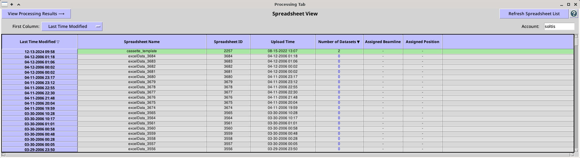
The Spreadsheets View currently displays the Last Time Modified, Spreadsheet Name, Spreadsheet ID, Upload Time and the Number of Datasets associated with a particular spreadsheet. If the selected spreadsheet is currently assigned to a beamline, the last two colums (Assigned Beamline and Assigned Position) will indicate the assigned beamline and the position of the cassette in the robot dewer.

To view the processing runs for a particular spreadsheet, highlight a row and click the "View Processing Results" toggle button or simply double click on the row. This will open a standalone Processing Tab for the selected spreadsheet.
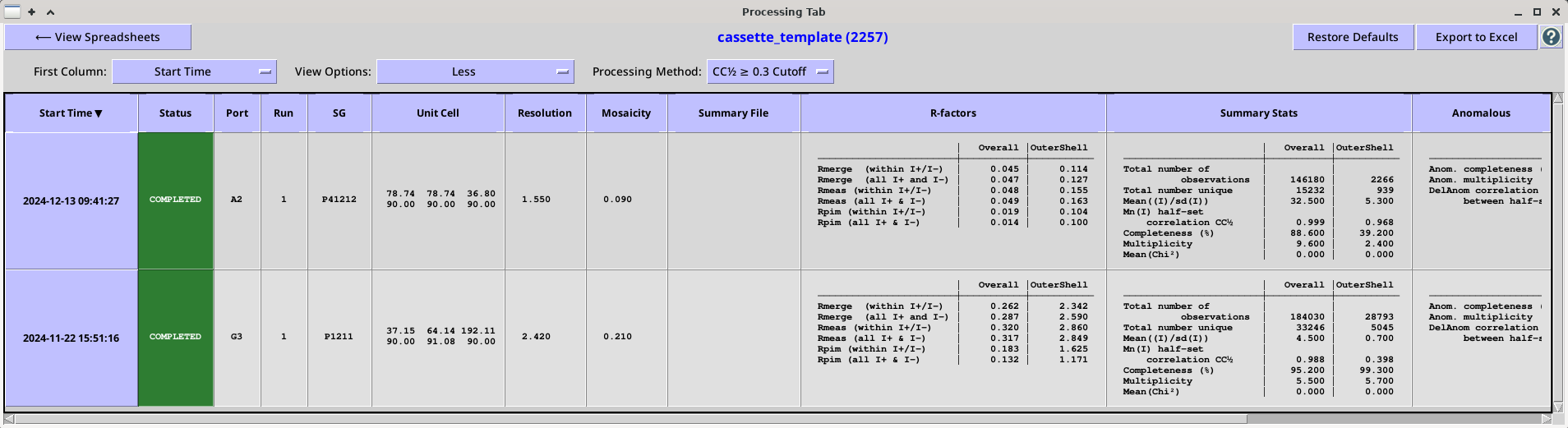
Figure: Processing Tab Results View.

Where Are My Data Located?

The data processing directories can be quickly accessed by clicking on the link listed in the "Processing Directory" column when in the View Options "More" or "All".

For those groups that have opted out, a symbolic link to the processing directories can be found in the image directory, for example:


	/data/{username}/mb_test/A5/autoprocessing_autoproc_8c562b 

How to Modify the Processing Script and Reprocess Datasets Manually

  1. Click on the Processing Directory link.
  2. Create a new processing subdirectory:
    
    	> mkdir new_processing_folder 
  3. Copy the processing script into the new folder:
    
    	> cp run-{cutoff}.sh new_processing_folder/my_new_run.sh
    	
  4. Open the new script in the geany or gvim text editor and modify the autoPROC launch string as needed:
    
    	> cd new_processing_folder
    	> geany my_new_run.sh
            

    CRITICAL - make sure to add the subfolder name after the -d argument or the script will not run! e.g.:

    
    	process [pre-existing arguments] -d .../new_processing_folder [rest of arguments]
            
  5. Save the new version and run my_new_run.sh:
    
            > ./my_new_run.sh
            

ICEflow Pipeline (autoPROC)

The intial version of ICEflow, deployed autoPROC v1.0.5 in a default configuration. Changes made to the pipeline, 3rd party software, configurations, input parameters, etc. are listed and documented in the next section.

Resolution Cutoffs

  • cc12 – Data are processed using a resolution cutoff corresponding to a target value for CC12 (~0.3) that is dynamically optimized by autoPROC.
  • isigi - Data are processed using a resolution cutoff corresponding to a value of I/σ(I) that is fixed at 1.5.

Programs and Output

  • autoPROC - the data processing pipeline. The general log files are written into the top directory:
    • out-{cutoff}.log - log file(s) for the entire automated processing run.
    • {cutoff}/summary.html - result summary in webpage format, can be viewed by running a web browser.

      NOTE: {cutoff}_summary.html files are also copied to the top folder.

    • {cutoff}/truncate-unique.mtz – final MTZ file containing integrated intensities and structure factors.
    • {cutoff}/truncate-unique.table1 - Table1-formatted merging statistics corresponding to the above MTZ file
    • {cutoff}/staraniso-alldata-unique.mtz - final MTZ file processed using ellipsoidal truncation to account for anisotropy.
    • {cutoff}/staraniso-alldata-unique.table1 - Table1-formatted merging statistics corresponding to the above MTZ file
    • NOTE: For STARANISO anisotropic analysis output files, see the anisotropic section in the summary.html file.

  • XDS – performs indexing, refinement, and integration. The input file XDS.INP - generated automatically by autoPROC - supplies the default parameters to the program and is based upon information stored in the header of the diffraction images (detector type and distance, oscillation start and range, number of images in the date set, etc.). The important output files from XDS can be found in the cutoff subfolders, which contain:
    • IDXREF.LP - the results of the automated indexing to find the unit cell parameters and an idea of what the crystal symmetry is.
    • INTEGRATE.LP - the full log of the processing.
    • CORRECT.LP - gives an indication of the data quality and resolution.
    • XDS_ASCII.HKL - contains integrated intensities.
  • POINTLESS – is run often during the workflow to analyzes the data for twinning, symmetry, and will identify the correct space group.
  • AIMLESS - takes the output from POINTLESS, calculates scale factors between all the images in the data set, applies the scales, and merges all the reflection data together to give an output file containing one copy of each reflection (the unique data set). While the key output from AIMLESS is included in the general autoPROC output file; the full log can be found in the {cutoff} directory.
  • CTruncate - reads the output from AIMLESS and attempts to put the data onto an absolute scale and generates structure factor amplitudes (F) from the reflection intensities (I). Its output can be found in the {cutoff} directory

References

  • autoPROC - Vonrhein, C., Flensburg, C., Keller, P., Sharff, A., Smart, O., Paciorek, W., Womack, T. & Bricogne, G. Data processing and analysis with the autoPROC toolbox. Acta Crystallographica D67, 293-302 (2011).
  • autoPROC - Vonrhein, C., Flensburg, C., Keller, P., Fogh, R., Sharff, A., Tickle, I.J. and Bricogne, G., Advanced exploitation of unmerged reflection data during processing and refinement with autoPROC and BUSTER. Acta Crystallographica D80(3) (2024).
  • STARANISO - Tickle, I.J., Flensburg, C., Keller, P., Paciorek, W., Sharff, A., Vonrhein, C., Bricogne, G., STARANISO @ http://staraniso.globalphasing.org/cgi-bin/staraniso.cgi Cambridge, United Kingdom: Global Phasing Ltd. (2016).
  • XDS - Kabsch, W. XDS. Acta Crystallographica D66, 125-132 (2010).
  • POINTLESS - Evans, P.R. Scaling and assessment of data quality, Acta Crystallographica D62, 72-82 (2006).
  • AIMLESS - Evans, P.R. and Murshudov, G.N. How good are my data and what is the resolution? Acta Crystallographica D69, 1204–1214 (2013).

ICEflow Versions and Release Notes

  • ICEflow-2.0.0 - released on 11/15/2025
    • New standalone Spreadsheet Viewer to view past results while on-line or off-line.
    • "Export to Excel" feature.
    • Changed from aimless.xml to autoproc.xml for display stats. Output now exactly matches autoProc summary.html file.
    • Fixed ambiguity for CC(anom) and added anomalous_signal/noise ratio.
    • Anisotropy calculation.
    • Anomalous detection and resubmission with anomalous flags set.
    • Multi-energy, inverse beam and wedge data set processing.
    • Removed "No Cutoff" jobs to free up CPUs.
    • Changes to the GUI:
      • New buttons: Export to Excel" and "View Previous Results".
      • Anisotropy column added.
      • "Potential anomalous signal detection and spawning new job" reported in Anomalous Signal column.
      • A clickable link that displays the header contents of the image file.
      • Slurm paramters added to the "All" view for troubleshooting".
      • Misc. fixes (spacing, widths, units, etc.).
  • ICEflow-1.5.0 - released on 03/19/2025
    • ICEflow jobs are now submitted to a queue using the Slurm workload manager.
    • Processing job submission parameters tweaked for optimal resource usage.
    • Major changes to the GUI:
      • A new status - "Pending" - appears for jobs waiting to run.
      • New columns added to the Layout, with two settings available to users.
      • A clickable link to a summary webpage file added.
    • autoPROC log parsing takes into account new formatting.
  • ICEflow-1.4.0 - released on 01/14/2025
    • Added data collection strategy calculation (iMosflm) to ICEflow packages
    • Strategy can be found on the Collect Tab
  • ICEflow-1.3.0 (autopPROC) - released on 09/12/2024
    • Added error extraction from logs and reporting in the Processing Tab.
    • Reorganized result reporting to database and UI.
  • ICEflow-1.2.1 (patch) (autopPROC) - released on 06/21/2024
    • Fixed issue where autoPROC could not index images collected with a vertical offset on a Pilatus detector.
    • Changed symlinks in data folder to point to the top processing folder.
  • ICEflow-1.2.0 (autoPROC) - released on 06/18/2024
    • Changed to a more descriptive convention for output folder: /data/{username}/{3rd_party_software}/{filename_prefix}_{run_number}_{date}_{time}/{cutoff}
    • The README file now contains explicit path to source data and image file template, for easier reference.
    • Documentation below edited to reflect these changes.
  • ICEflow-1.1.0 (autoPROC) - released on 06/12/2024
    • Fixed an issue where both cutoff versions output data with a CC1/2-based resolution cutoff; the I/σ(I)-based cutoff is now enabled.
    • Added a no-cutoff option as documented below.
    • The summary.html files are now copied to the top folder for easier access.
  • ICEflow-1.0.0 (autoPROC) - released on 06/05/2024
    • Initial release, with only autoPROC pipeline enabled.

Pipelines Running before the Inception of ICEflow (before 6/5/2024)

For the SSRL pipeline (and the xia2 test pipeline), look in the image file directory for the symbolic link to the directory with the processed data (these links will all begin with 'autoprocessing'). The processing directory contains the README file that describes the pipeline used for data processing. If you can't find what you're looking for, contact your user support staff member.


More information on the software supported by the SSRL-SMB Macromolecular Crystallography division is available on our software webpage.