Scan Tab
Overview
The Scan Tab is used for energy and excitation scans. The
energy (MAD) scans are used to select the appropriate wavelengths for
anomalous dispersion experiments (optimized SAD
and MAD). The excitation scan is useful to identify and verify the
presence of anomalous scatterers in the sample
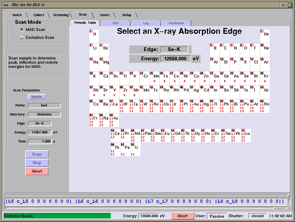
[Fig 1. The Scan Tab in Blu-Ice]
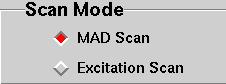
MAD Scan
- This mode is used to scan the x-ray energy against the
fluorescence emitted by the sample and subsequently determine the optimal
energies for MAD data collection.
[Fig 2. Scan Mode and Scan Parameter
Menus]
Selecting
an X-ray Absorption Edge
- The desired absorption edge can be selected from the Periodic Table tab.
- Select an edge by clicking on a particular edge
(K, L1, L2,
L3) and press the Scan
button.
|
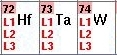
- For some elements, such as those shown to the left, you
can select different edges--
L1, L2, L3. As a rule of
thumb always select L3 for heavy elements; however, if
this edge is not accessible at the beamline, try scanning the
L2 edge instead. The L1 edge, on the other hand is usually to
small to provide a good dispersive signal, and a SAD (instead
of MAD) experiment above this edge is recommended if neither
the L2 nor the L3 edges are accessible. Consult the support staff for
help with selecting the edge.
|
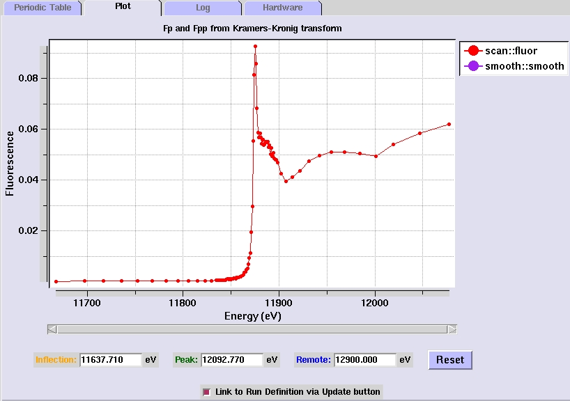
Analyzing and examining the Fluorescence Scan
- The program autochooch automatically calculates
the anomalous scattering factors from the fluorescence
data. The f" and f' plots are displayed in the Plot
tab, as well as the suggested peak (maximum f") , inflection
(minimum f') and remote (high f" and f') energies for
MAD data collection.
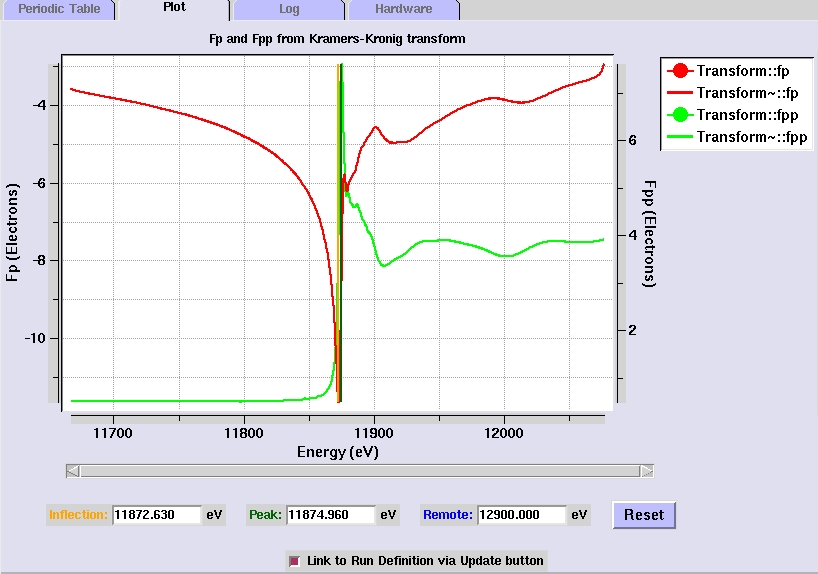
[Fig 4. Plot of f" and f'
values calculated from the fluorescence scan]
- The selected
energy values can be adjusted by moving the vertical cursors
(the blue line in Figure 4). The cursors can be moved by
clicking on them with the middle mouse button. Right clicking
on the cursors will give options to change the cursor color,
cursor thickness, and to delete the cursor. This will update
the energy values selected for data collection
- Checking The Link to Run Definition via Update box
allows exporting the energy values into the collect tab (this
is the default after a successful scan). Pressing the Update button in the Collect
Tab will then import the energies for MAD data
collection.
- You can
display the raw fluorescence counts by clicking the right
mouse button on either side of the plot and selecting a new Y
axis label.
- By clicking the right mouse button on the transform
or any other lines in the plot, users can change various
parameters like line color, line thickness, symbol shape and
color, etc.
- Placing the mouse over the plot line will display
the x and y coordinates for each point. This is useful to find
out the f' and f" values for energies other than the
ones written out by autochooch.
The f' and f" for the autochooch energies can be obtained from the
Log tab or the summary
file. If you use a different remote wavelength to the one
selected by the software, you can get the f' and f"
values from these
tables.
- To zoom in the plot, left click on a point of the
plot window, hold down the mouse key and drag the mouse to
define the zoom rectangle. The zoom level changes after
releasing the mouse button. Right clicking on the plot window
displays a menu with the option to zoom out.
Output files
The following files are written out after successful completion of
a fluorescence scan:
- name-scan: Contains the raw fluorescence readings
- name-smooth_exp.bip and name-smooth_norm.bip: Intermediate
files from autochooch
- name-fp_fpp.bip: Anomalous scattering factors (f" and f') calculated by autochooch
- name-summary: Summary of the scan, including the values for the
peak, inflection and remote wavelengths and the
f" and f' values for each of them
A summary of the scan is also displayed in the Log tab
Saving, reading and printing fluorescence scans
Right-clicking the mouse on the plot window opens a menu which
allows saving, printing and opening fluorescence scan files.
- The print option will send the current scan plot to
the default printer.
- The open option allows to read in previous scan
files. The program will open a file browser to help locate the scan files.
- The save option has been superseded by the automated
generation of output files. The program
will prompt for the output file name and will write out a single bip
file containing the fluorescence counts, processed counts and f"
and f' values for each energy.
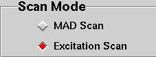
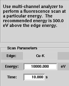
Excitation Scan
While MAD scan measures the fluorescence counts from a
single element by changing the energy, the excitation scan measures
the fluorescence counts from any element present in the sample with an
absorption edge below the excitation energy. Excitation scans are very
useful for the identification of heavy elements in a crystal. They
take less time than the MAD scans and thus are a faster way to
determine the presence of a heavy atom derivative/ligand in the
sample.
[Fig 5. Excitation Scan Mode]
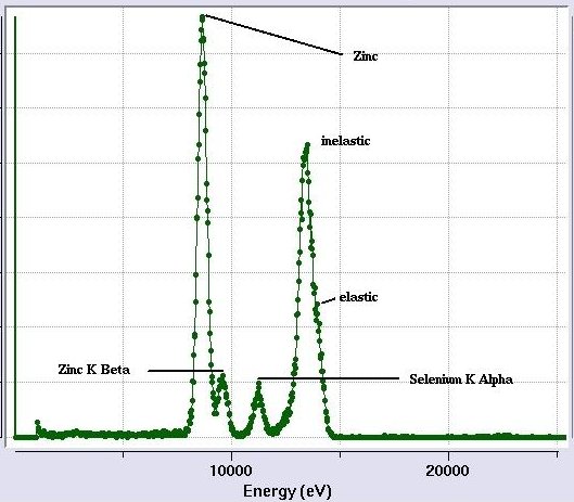
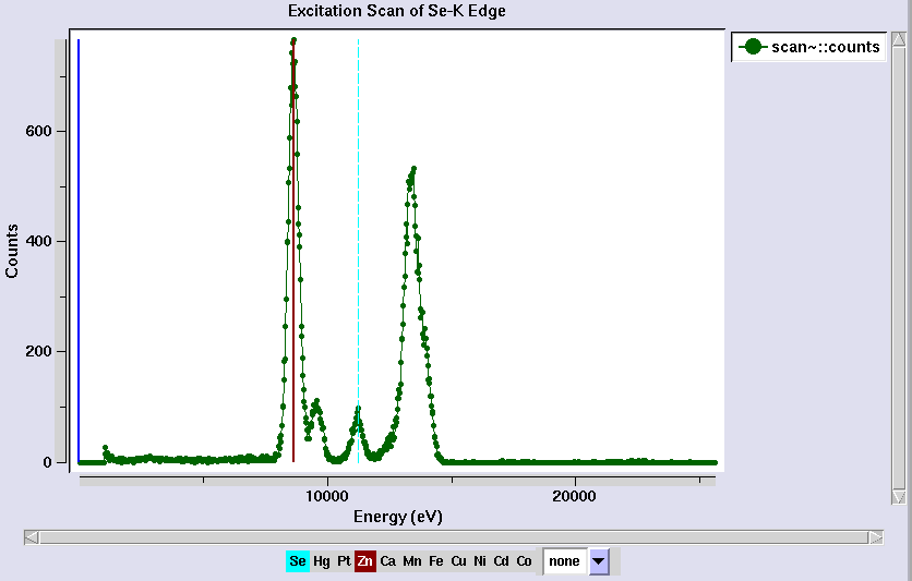
[Fig 7. Fully interpreted excitation scan.
The elastic and inelastic peaks are not separated because of the detector resolution.
The K-beta peak for Se is relatively small in this sample and it disappears into
the tail of the next peak at higher energy.]
Pitfalls and caveats
Sometimes emission peaks for different elements
will overlap. In this case, you need to use common sense to identify the
element. Could one of the elements be present in your crystal as a derivative, ligand or part of the
buffer?. If not, the chances are that the element is something
commonly found in proteins (the right-most elements listed under the
plot) and not a rare-earth or a heavy transition metal.
If you find many different strong emission peaks that you don't
expect (Cu, Ni, Fe), double-check that you are not hitting the metal
pin. Very weak peaks may also originate from a source other than the
sample (beamline components or sample holders; for example, Zn emission
has been observed from empty loops, Pb from glass capillaries; Fe can
be present in the fluorescence Be window. It is a good idea to repeat
the excitation scan in absence of the sample and verify that the
peaks disappear too.
Appendix: Absorption edge and main emission line energies
Strongest emission lines for the most common elements present or
introduced in biological macromolecules. (Emission and excitation energies
in eV).
| Element
| Fluorescence
| Excitation
energy
| Edge accessible
for MAD
|
|
|
| Mg
| 1254
| 1303
| No
|
| P
| 2014
| 2145
| No
|
| S
| 2308
| 2472
| No
|
| Ca
| 3692
| 4038
| No
|
| I
| 3937
| 4557
| No
|
| Xe
| 4110
| 4786
| No
|
| Sm
| 5636
| 6716
| 12-1,12-2,9-2
|
| Mn
| 5899
| 6539
| 12-1,9-2
|
| Fe
| 6403
| 7112
| 12-1,12-2,9-2,14-1,7-1
|
| Ni
| 7478
| 8333
| 12-1,12-2,9-2,14-1,7-1
|
| Cu
| 8048
| 8979
| 12-1,12-2,9-2,14-1,7-1
|
| Ta
| 8146
| 9881
| 12-1,12-2,9-2,14-1,7-1
|
| W
| 8398
| 10207
| 12-1,12-2,9-2,14-1,7-1
|
| Zn
| 8639
| 9659
| 12-1,12-2,9-2,14-1,7-1
|
| Os
| 8912
| 10871
| 12-1,12-2,9-2,14-1,7-1
|
| Ir
| 9175
| 11215
| 12-1,12-2,9-2,14-1,7-1
|
| Pt
| 9442
| 11564
| 12-1,12-2,9-2,14-1,7-1
|
| Au
| 9713
| 11919
| 12-1,12-2,9-2,14-1,7-1
|
| Hg
| 9989
| 12284
| 12-1,12-2,9-2,14-1,7-1
|
| As
| 10544
| 11867
| 12-1,12-2,9-2,14-1,7-1
|
| Pb
| 10551
| 13035
| 12-1,12-2,9-2,14-1
|
| Se
| 11222
| 12658
| 12-1,12-2,9-2,14-1,7-1
|
| Br
| 11924
| 13474
| 12-1,12-2,9-2
|
| Kr
| 12649
| 14326
| 12-1,12-2,9-2
|
| U
| 13615
| 17166
| No
|
| Sr
| 14165
| 16105
| 12-1,12-2
|
|