|
MulticrystalThe Multicrystal tab provides tools for combining diffraction data from multiple crystals into a single merged dataset. The scaling tool displays numerous parameters and filters for excluding outlier datasets. Create a New ProjectThe Create New tab (Fig. 1) allows you to create a multicrystal project from two different types of sources:
Once the datasets have been selected, enter a project name and click Create. Note: projects are automatically created for the BluIce multicrystal data collection mode and will automatically appear in the Projects list. Figure 1. The Create New tab can be used to create a multicrystal project. List ProjectsThis tab (Fig. 2) provides a list of all your multicrystal projects and associated information:
Use the Options dropdown to open projects in the Scaling Tool or to delete them. 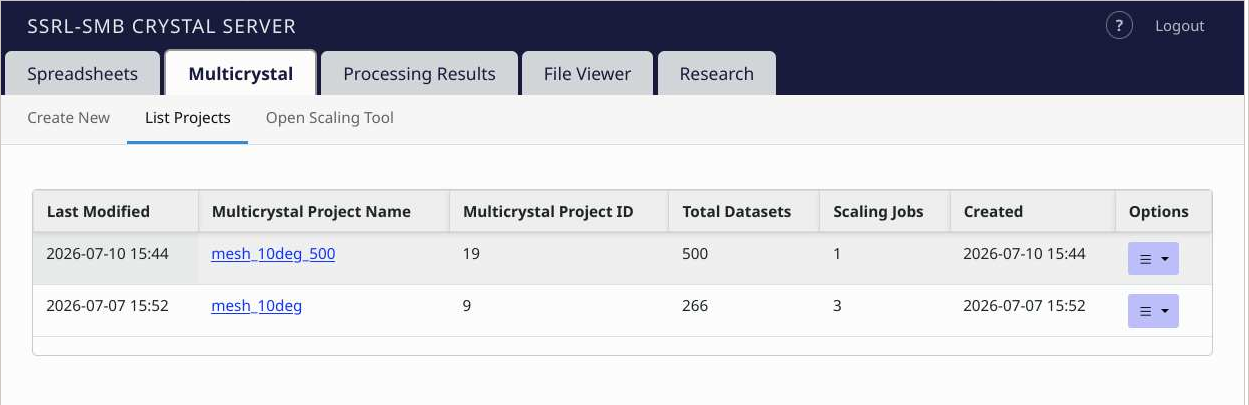
Figure 2. The List Projects tab displays all your multicrystal projects and relevent project information. Multicrystal Scaling ToolThe Scaling Tool is the main interactive interface for configuring and running aP_scale jobs (Fig. 3). It has several sections: a main control bar, a panel for filtering out datasets, unit cell distribution, data coverage, an advanced options section. A panel to display intensity correlations for uncovering nonisomorphism and a table listing each dataset and associated processing parameters. 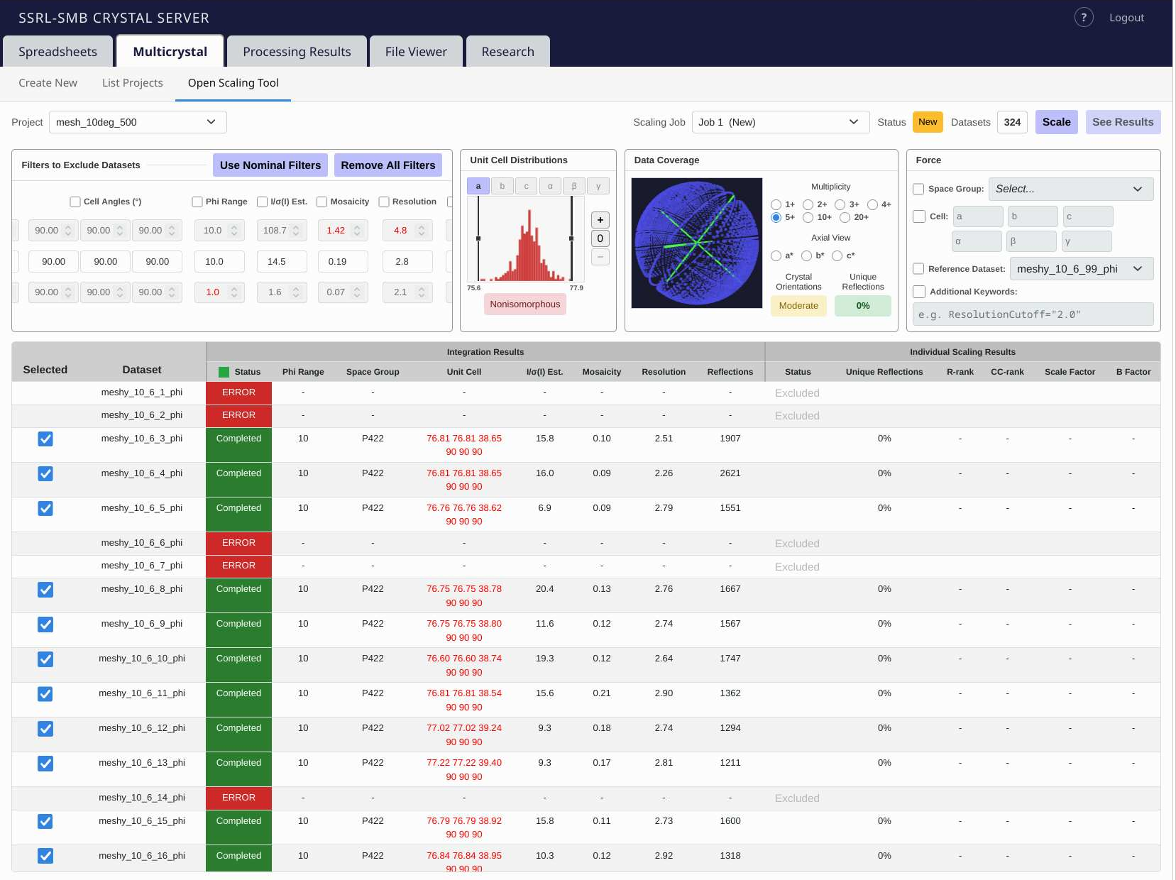
Figure 3. The multicrystal scaling tool displays processing results from individual datasets which can be filtered before merging with aP_scale. Control BarThe main control bar (Fig. 4) is used to select a multicrystal project, create scaling runs, and submit scaling jobs to the compute cluster. 
Figure 4. The main control bar for selecting projects and creating/submitting scaling jobs. A list of availabe multicrystal projects are shown in the Project dropdown menu (Fig. 5). Projects can be selected or removed and addtional datasets can be added using this menu. In addition, missing parameters (spacegroup, cell, ISa...) can be refreshed from autoPROC directories. This is useful when parameters are missing, stale, or if the data has been reprocessed. 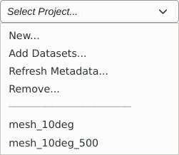
Figure 5. The Project menu is used to select or add datasets to existing multicrystal projects.. The Scaling Job menu displays a list of scaling jobs and their status (Fig. 6). Prvious scaling jobs can be selected or removed. Selecting New... will create a fresh scaling job and it can be based on any previous scaling job or it can be based on the unscaled integration data. Note: for scaling jobs that have been submitted or have compelted, the tool is completely locked out. To make changes, a new scaling job must be created 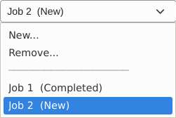
Figure 6. The Scaling Job menu is used to select or create new scaling jobs. The New Job button will create a new scaling job increamenting the jib number by 1 (only 1 new job can be created at a time). Filter PanelThe filter panel (Fig. 7) is used to apply quality-based filters to exclude poor quality datasets. The corresponding checkbox must be checked for the filter to be applied. 
Figure 7. The Filter panel provides a way to exclude datasets based on processing parameters. Each parameter shows the minimum, average and maximum values for the selected datasets. A red value indicates it is outside "nominal" limits. The Min and Max arrows can be used to manually narrow or expand a range or a value can be entered manually. Note - depending on your window size you may have to hover over the panel to see the horizontal scroll bar to access all available output parameters. Scaling output parameters (dereived in comparison to other datasets) will also be available for filtering after the first scaling job has completed. These include (R-rank, CC-rank, Scale Factor, B Factor). The Use Nominal Filters button applies a nomnal set of limits and the Remove All Filters button removes all filtering. Integration parameters that can be used for filtering datasets:
Individual Scaling Results that can be used for filtering datasets:
Unit Cell DistributionThe Unit Cell Distribution panel (Fig. 8) provides an interactive histogram for each unit cell parameter (a, b, c, α, β, γ) that can be used for excluding datasets. Drag the min/max sliders to exclude outliers and narrow the range. Click "+" icon to expand the view. Nominal definitions indicate the selected range is isomorphous, moderate or nonisomorphous. 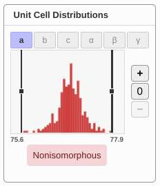
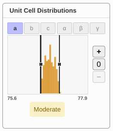
Figure 8. The interactive Unit Cell Distribution panel provides a histogram of unit cell parameters (left) that can be filtered to remove outlier datasets (right). Data CoverageThe Data Coverage panel (Fig. 9) provides a 3D visualization of the estimated reciprocal space coverage for the selected datasets. The minimum multiplicity level can be set (1+, 2+, 5+, etc.) and the sphere can be viewed along or rotated about the reciprocal axes (a*, b*, c*) to inspect coverage. In addition, the range of different crystal orientations is displayed (Random, Moderate and Clustered). The amount of unique reflections (no overlapping reflection) is also displayed (Few, Moderate, Many). 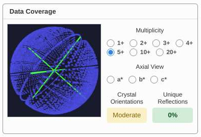
Override Panel (Advanced)The Override panel (Fig. 10) allows one to override specific parameters including adding any valid keyword to the aP_scale run. 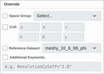
Figure 10. The advanced Override panel is used to override parameters or aP_scale keywords. Parameters that can be overriden: Intensity CorrelationThe Intensity Correlation panel (open by clicking on the arrow in the panel) can be used to determine if there is nonisomorphism even when there is no significant differences in unit cells (Fig. 11). A heatmap is produced correlating each dataset with each of the other datasets (Fig 12). This map is then used to create a dendogram (Fig. 11) linking the datasets together based on their correlation coeficients. Once a isomorphous cluster is identified, the other datasets can be excluded for scaling using the Select Cluster column. The input parameters include:
The CC cutoff can also be selected by grabbing the red dashed line with the mouse and moving it to a given CC value. 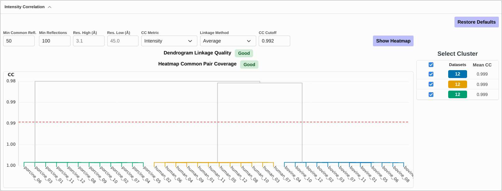
Figure 11. The Intenisty Correaltion panel can help determine if there is nonisomorphism accross datasets. 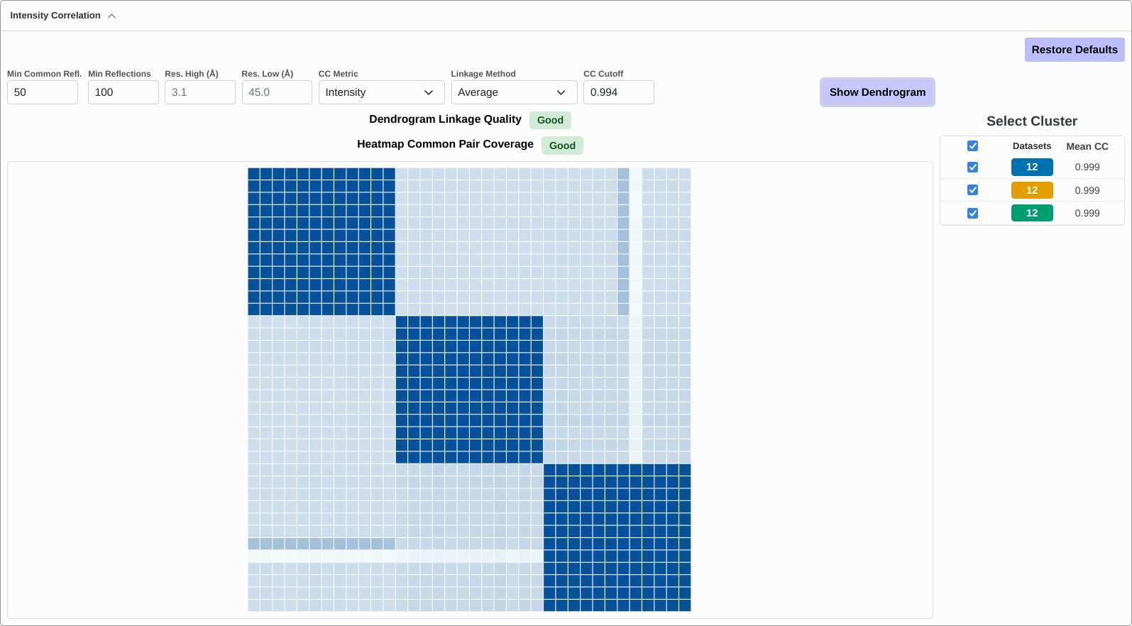
Figure 12. The Intenisty Correlation heatmap used to determine if there is nonisomorhism accross datasets. Figures 11 and 12 show an example of true nonisomorphism. There are three different stuctures with subtle differences that cluster in the dendogram. There are also indicators for how well the map and dendogram can be trusted. In this example, both indicators are "Good". When the heatmap has many missing CC's due to the lack of overlaps or if the denogram linkage has issues, the indicator will read "Moderate" or "Poor". In those cases, the data may not be of high enough quality to produce trustworthy clustering. When uncertain, scale the individual clusters and compare the processing results to the results for processing all the clusters as one dataset. A typical dendogram for isomororphous crystals is shown in Fig. 13. The tell is the hieght of the connections. Unike Fig. 11, there are no large vertical gaps between clusters. 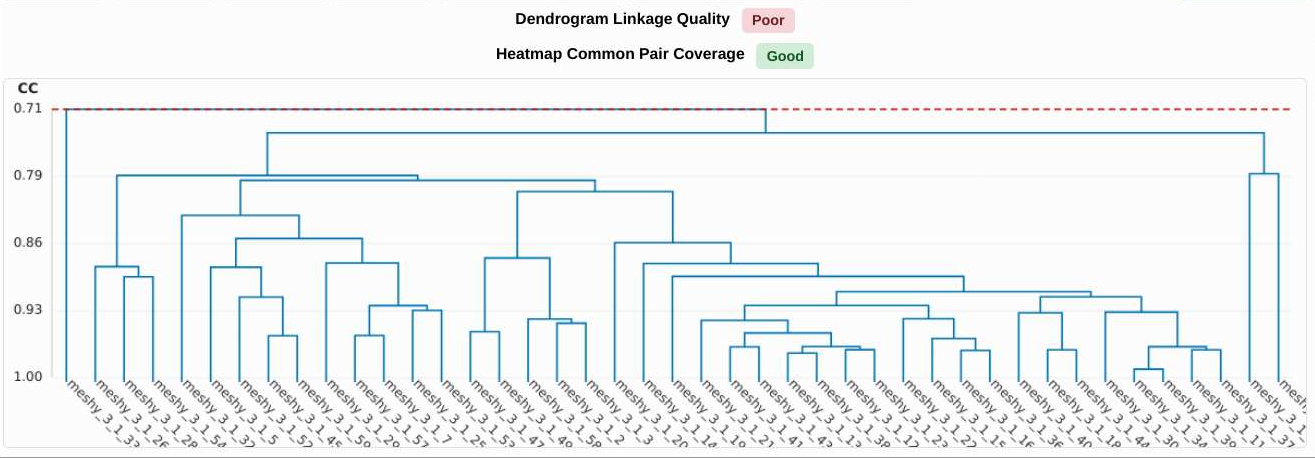
Figure 13. A typcai dendogram of isomorphous crystals. By selecting Anomalous under the CC Metric drop down menu, datasets can be clustered based on their anomalous signals. Dataset Display TableThe dataset display table (Fig. 9) shows the results of the individual dataset integration runs,
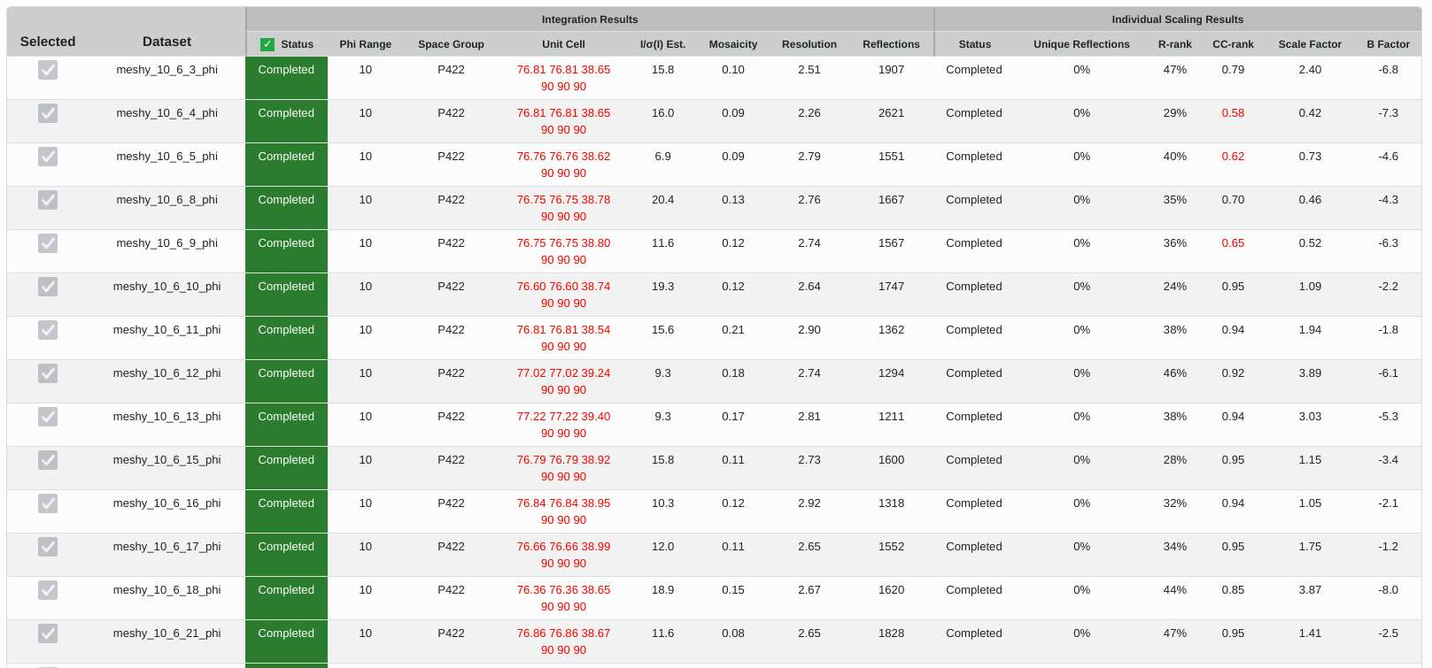
clustering results based on intensity correlations (if datasets hve been excluded using the Instensity correlation panel), as well as the results of the scaling run.
Figure 9. The display table of datasets with associated processing parameters. The Dataset display table lists every dataset with Integration Results: After the first scaling run, Individual Scaling Results are also displayed: Values that are highlighted in red are outside the "nominal" limits. Manually select or deselect datasets for scaling using the checkboxes on the left side. Use the green box in the Status column header to remove datasets from the display that had produced an error during integration (datasets with errors are excluded from the selected list wehter they are displayed or not). |
||
|
|
||
| Technical questions: Webmaster
Content questions: Mike Soltis |
||
| Last modified:Monday, 17-Aug-2026 18:13:19 PDT. | ||