Table of Contents
Data Collection Strategy with iMosflm
The steps below provide a brief description of how to use imosflm to generate a strategy for the optimum crystal rotation range and step size to use for x-ray diffraction data collection. These directions assume that you have collected two test images from your crystal, 90° apart. If you haven’t done this, please follow the directions in the BluIce instructions to collect the two "snapshots".
NOTE: Make sure to connect to one of the data processing servers at SSRL as described in the User Guide; imosflm and other processing programs are not installed in the NX servers and beamline control machines.
Instructions
- Navigate to the subdirectory in your
/data area where you have collected the two test images.
- Launch the iMosflm GUI by typing
imosflm
- Click the fourth small icon at the top left (“Add Images”) (Figure 1)
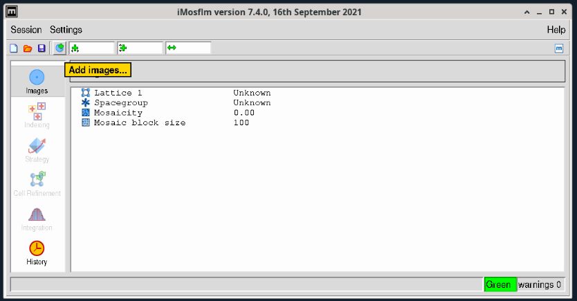
Figure 1. iMosflm GUI with "Add Images..." button indicated.
- Select one of the test images and click OPEN.
- The image will open in a separate window – you can minimize this if you wish.
- Select the large “Indexing” task icon from the lefthand vertical toolbar. Indexing will run automatically on the two images (Figure 2) and a Mosaicity Estimate window will pop up. You can close this.
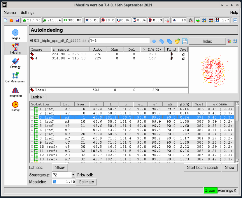
Figure 2. iMosflm GUI Autoindexing window.
- A Bravais Lattice and cell are selected in the table at the bottom. (If the suggestion is incorrect, you can override the selection if necessary by clicking on a selected line in the table).
- Select the large “Strategy” task icon from the lefthand toolbar, then click the “Auto-Complete” button on the upper right and click OK in the small dialog window that pops up. The data collection strategy is then calculated (Figure 3).
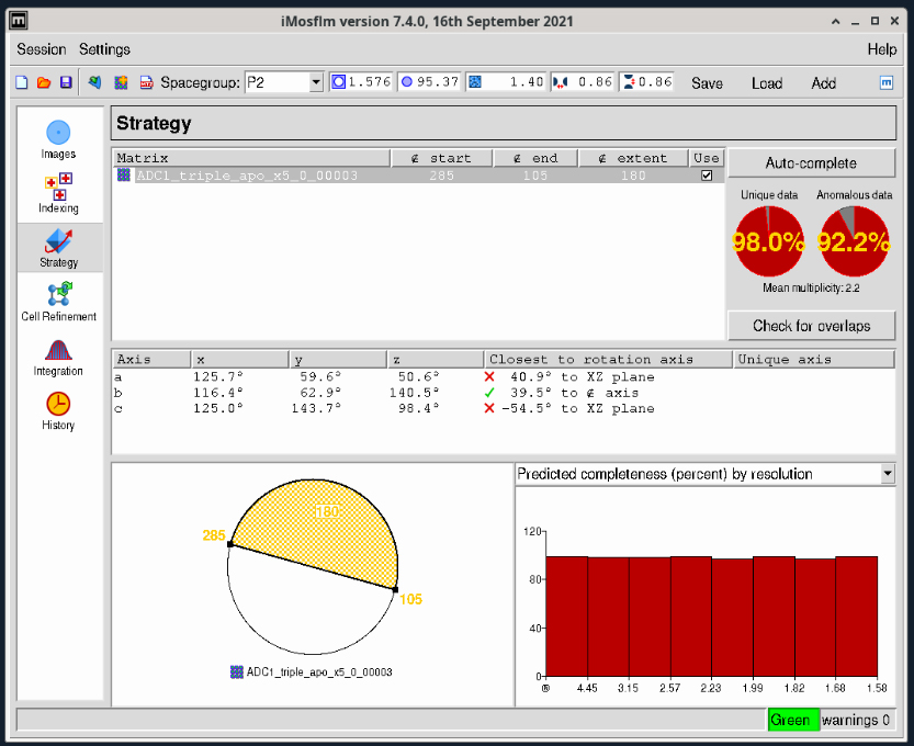
Figure 3. iMosflm GUI Strategy window.
- The two circular red plots at the upper right show you the estimated completeness for the data collection range that is displayed at the lower center of the window (white and yellow circle). This diagram tells you the starting and ending angles for data collection segment colored yellow – in Figure 3 these values are 285° and 105° respectively. You can click on the small square box at either end of the yellow segment to adjust the starting and ending angles. The selected segment will turn red as shown in Figure 4. The new starting and ending angles are 270° and 180° degrees respectively. You can use these values in the Blu-Ice Collect tab to set up your data collection.
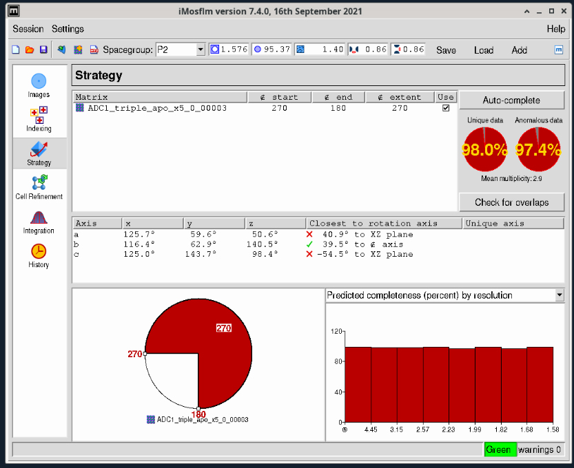
Figure 4. iMosflm GUI Strategy window - strategy adjustment.
- In cases where you have a very long unit cell axis, overlapping reflections can be an issue. It is always useful to check the potential overlaps by clicking the “Check for overlaps” button just below the two red completeness plots on the right. This will bring up a dialog box (Figure 5) where you can select the desired oscillation angle. Initially this will be ‘Variable’ but you should select the oscillation range you will use for collection (with the Pilatus and Eiger detectors we recommend between 0.1-0.2° – what is termed “fine-slicing”). Choosing 0.2° in this case gives no overlaps as shown in the plot at the bottom right in Figure 6.
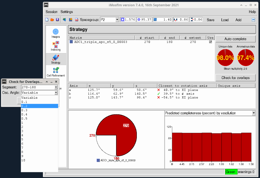
Figure 5. iMosflm GUI Strategy window - check for overlaps.
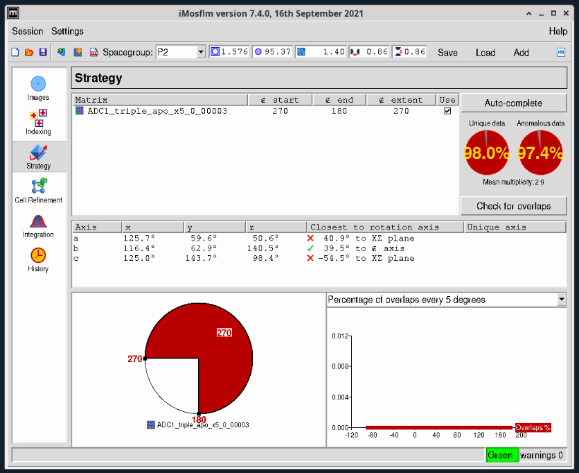
Figure 6. iMosflm GUI Strategy window - adjusted strategy with no overlaps.
- To optimize your exposure time, we next recommend entering your iMosflm strategy into the Blu-ice collect tab, and then using the
raddose3D dose calculator.
Quick data processing with iMosflm
This is a brief description of how to use imosflm to quickly process and scale data to get an idea of the quality of the
data. For a more complete description of the program and its advanced features, visit the iMosflm Tutorial site at MRC-LMB Cambridge.
- Start by logging in to one of the data processing servers at SSRL as described in
the User
Guide. Mosflm and other processing programs can be CPU and memory hungry and therefore are not installed in the NX servers and beamline control machines.
- Create a subdirectory in your
/home or /data area where you want to store the results (you can also use an existing directory) and use the cd command to go to that directory, eg:
 cd /data/username
 mkdir MOSFLM-DEMO
 cd MOSFLM-DEMO
- Launch the GUI by typing
"imosflm" in that directory. When the GUI appears, start by creating a new session by clicking on the top left icon; you can hover with the mouse over the icons to find out what they are (Figure 7.). Creating a new session will allow you to see the results and add more files later on.
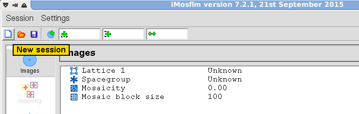
Figure 7. iMosflm GUI - new session.
- Next, add the images in the data set; click on the 4th icon. You can use the navigation icon to select the directory in your /data area, type the directory name in the input window or a mixture of both to locate your images (Figure 8).
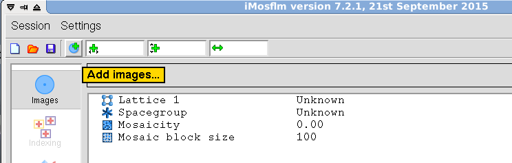
Figure 8. iMosflm GUI - Add Images.
- Then, click on one of the images (usually the first one) and the "Open button" (Figure 9). This will import all the images with the same root name. The program will also open the selected image in a separate window.
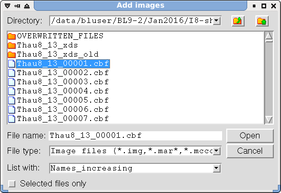
Figure 9. iMosflm GUI - select image range for import.
- You can use the "masking tool" and "circle fitting" in the image display window to mask out the beamstop shadow (Figure 11). The pixels in the detector seams have a special value and the software ignores them so you do not have to do anything about them.
- Go back to the main window and click on the "Autoindex" task icon (Figure 12). The program will select automatically the optimal images to autoindex and default parameters. After autoindexing, it will select a space group (you can override it) and provide an estimate for the mosaicity.
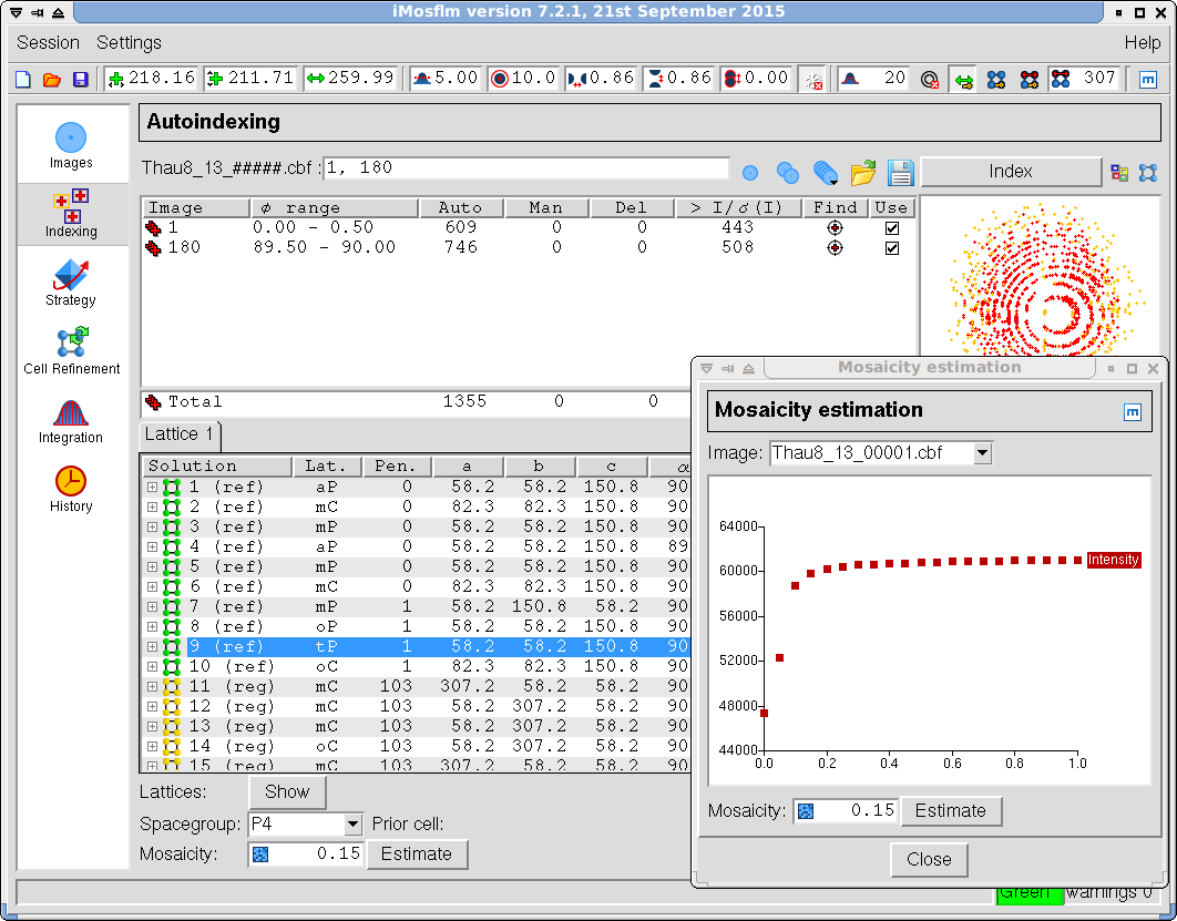 Figure 12. iMosflm GUI - Autoindexing.
|
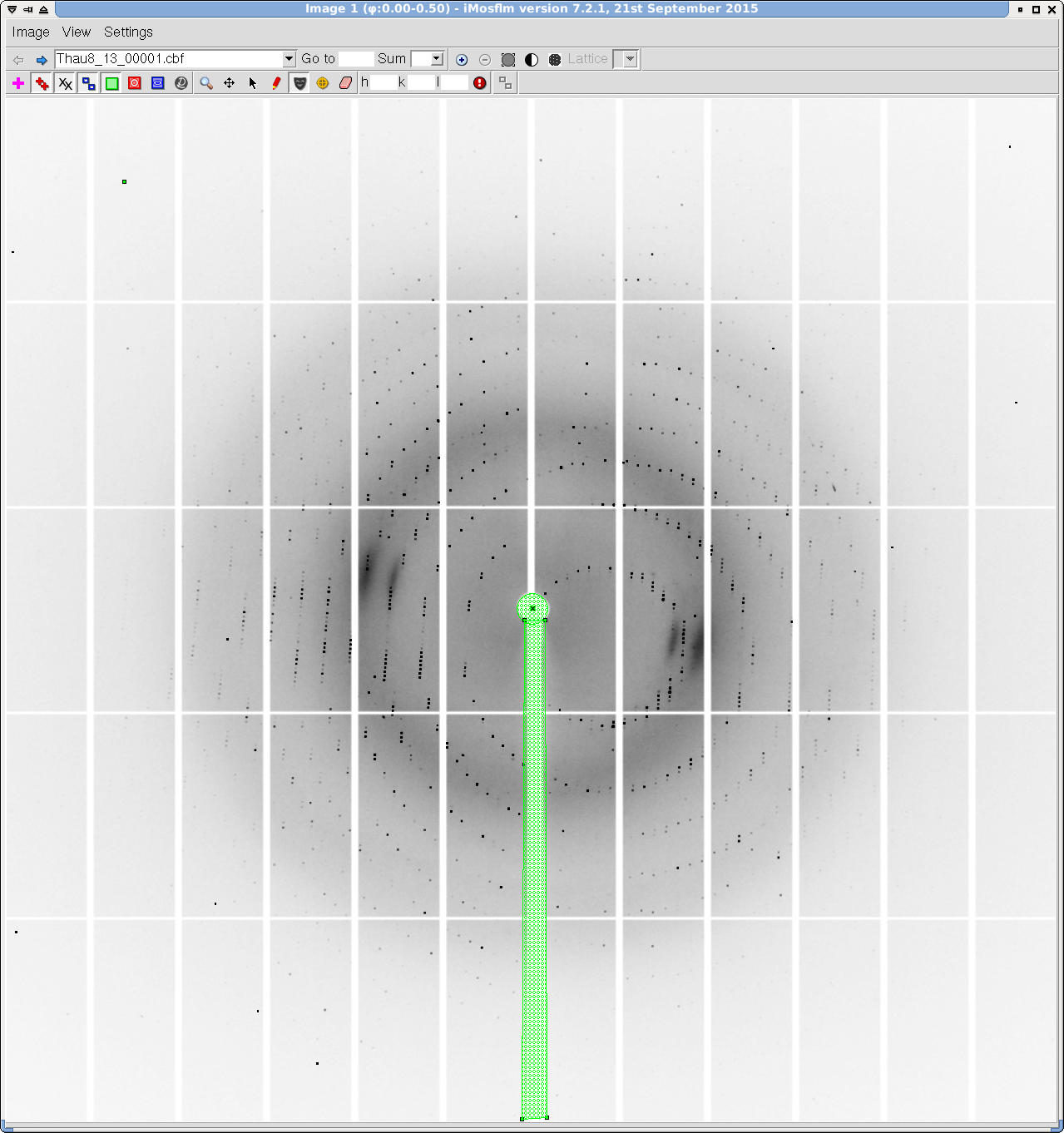
Figure 11. iMosflm GUI - Image display and masking.
|
- Next, refine the unit cell (Figure 13). In principle you can refine the unit cell during postrefinement, but refinement will be more stable if you do this step first. Once the program has selected the defaults, click on the "Process" button. The program will display the refined parameters for all the images. They are usually in two different wedges, so some discontinuity in the parameters is expected. Inspect the image display to make sure that the predictions match the position of observed spots.
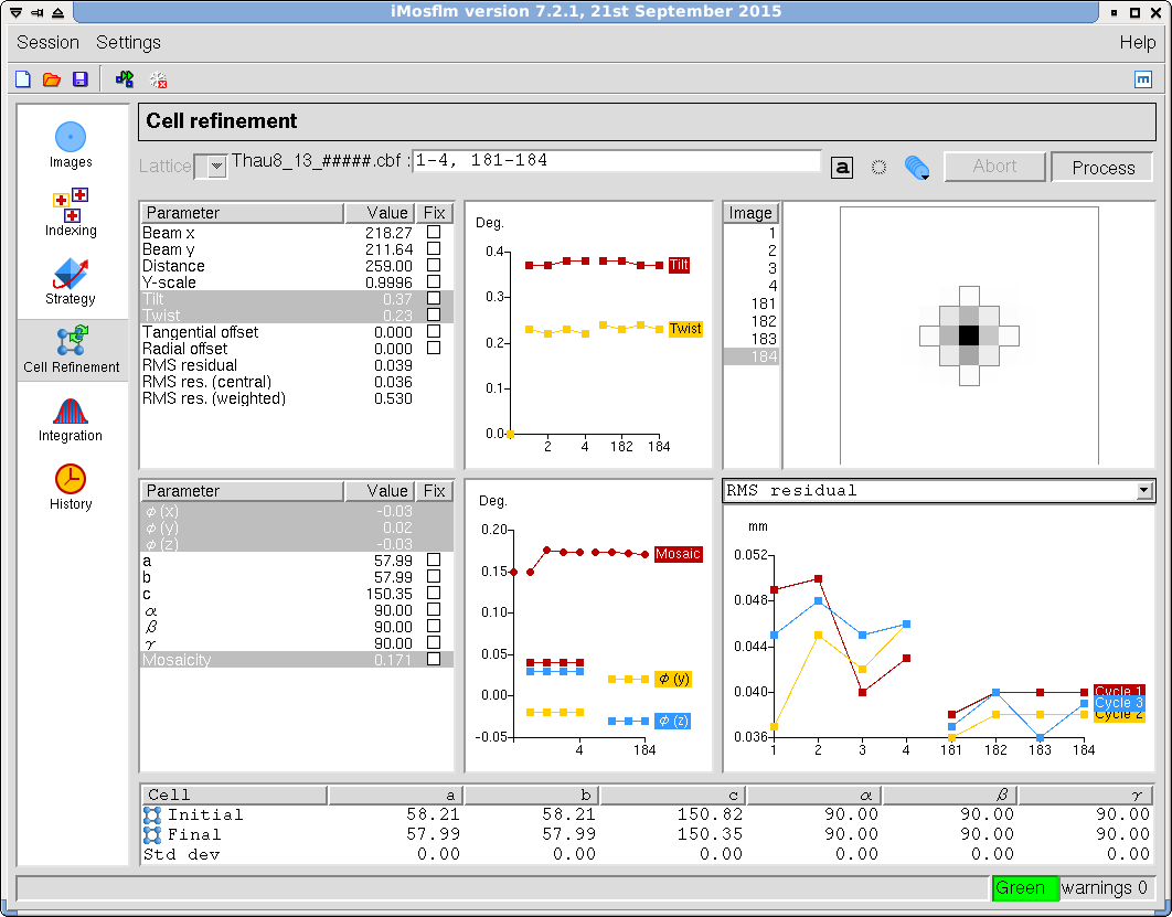
Figure 13. iMosflm GUI - Cell Refinement.
- Select the integration task to integrate and postrefine the images (Figure 14). Note that the program will fix the unit cell parameters by default. The program will display the results as integration and refinement progresses.
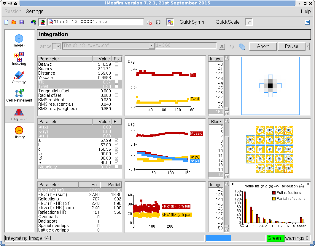
Figure 14. iMosflm GUI - Integration.
- Inspect the results. If your data are reasonable, you may still see some warning messages about the processing, which you may want to inspect eventually. Poor refinement parameter and integration statistics and critical error messages suggest that there is a problem with the data or the processing itself. If no errors are reported, press the "QuickScale" button to run symmetry analysis, scaling, merging and data truncating. This may take some time depending on how many images and reflections you have. After a while, the results will be displayed in a separate window and you will be able to make an assessment about the quality of your data set.
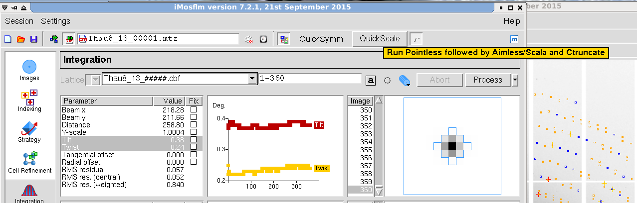
Figure 15. iMosflm GUI - Integration.
- The log and output files from all the steps of the processing will be stored in the directory you are running the program from. All the output files are written in mtz format. Files generated by the program are given a unique name based on the time and date or in the root name of the input images. Here is a list of the files:
mosflm.lp, .mat and .sum files: contain a detailed processing log, orientation matrix and processing summary.ANOMPLOT, ROGUEPLOT, ROGUES, NORMPLOT, CORRELPLOT and SCALES are auxiliary and plot files generated by Aimless.- The
pointandscale log contains the Pointless, Aimless and CTruncate logs.
- The
mtz file of the form {image_name}.mtz is the integrated intensities from mosflm. The pointless_{image name}.mtz file has unmerged sorted reflections in the correct space group. aimless_{imagename}.mtz has scaled and merged intensities and ctruncate_{image name}.mtz contains the intensities and calculated amplitudes (a "unique" version of this file, with a test (rFree) set selected, is also written out).
|