|
Run Dose Estimate
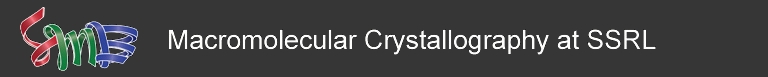
The Run Dose Estimate window in the Collect tab provides information about X-ray absorption during data collection. The window displays experimental Dose Limits based on the type of experiment being performed, a calculated Predicted Dose based on crystal parameters and data collection Run parameters, and an estimate of the Exposed Dose as the experiment proceeds (Fig. 4).
Figure 4. The Run Dose Estimate window (highlighted in orange) shows the X-ray Dose Limit and displays a Predicted Dose based on the sample crystal and the Run parameters. This example displays a Predicted Dose estimate that exceeds the limit for data collection at room temperature. (click to enlarge). The Dose Limit is defined as the dose which reduces the sample to half it's diffracting power or the loss of useful anomalous signal. The Dose Limit can be toggled by clicking on the Limit (blue indicates a toggle). Current options include:
The Predicted Dose (the Average Diffraction-weighted Dose) is calculated using Raddose3D. RADDOSE3D is also a supported program that can be run independently from the command line. The Exposed Dose is an estimate of how much dose the crystal has absorbed once data collection is running or has finished. The Predicted and Exposed Dose values will turn red to indicate a warning that they exceed the Dose Limit (Fig. 4). Note: The Predicted and Exposed Doses only apply to individual Runs since a translation of the sample to an unexposed area is assumed between Runs. If the crystal is exposed in the same position over multiple Runs, the total Predicted and Exposed Dose will be the sum of the doses for each Run.
Default Crystal Parameters
By default, a Predicted Dose will be calculated based on a number of Default assumptions:
Warning: If the above assumptions do not adequately describe your crystal, the predicted dose will likely be underestimated which can lead to an over-exposure of your sample. In this case, use the X-ray Dose and the Crystal Size sub-tabs to enter the appropriate sample information (see below).
X-ray Dose Sub-Tab
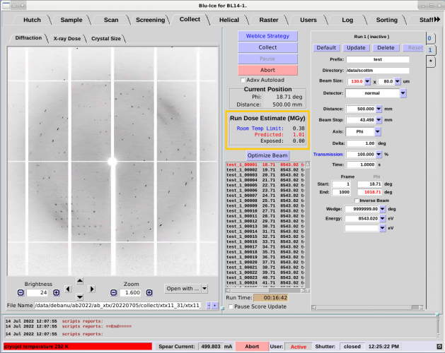
Relevant information about the mounted sample will yield a more accurate Run Dose Estimate. Sample parameters can be modified in the X-ray Dose sub-tab (Fig. 5).
Figure 5. Crystal parameters in the X-ray Dose sub-Tab (click to enlarge).
Unit Cell, Monomers and Residues
The unit cell can be specified as well as the number of monomers in the unit cell and the number of residues in each monomer. Alternatively, the molecular weight of the monomer can be specified by clicking on the "Number of Residues" parameter (blue indicates a toggle).
Heavy Atoms
The type and number of heavy atoms in each monomer can be specified (Fig. 6). For example, four iron and six selenium atoms in the monomer would be entered in the following manner: Fe 4 Se 6
Solvent Content
The percentage of solvent content can also be specified as well as the heavy atom concentrations in the solvent. The type and concentration (mmol/l) of each heavy atom type in the solvent can be specified (Fig. 5). For example, concentrations of 100 mmol/l of P and 350 mmol/l of S and 50 mmol/l of Zn would be entered in the following manner: P 100 S 350 Zn 50 Note: Atoms lighter than oxygen should not be included. Once the Dose Parameters in the X-ray Dose sub-tab have been entered, click on "Apply" to update the Predicted Dose Estimate. Values highlighted in red will be updated and a new Predicted Dose will be calculated. Use the Cancel button before clicking Apply to discard changes to the parameters. Note: The X-ray Dose sub-tab parameters apply to the crystal that is currently mounted on the goniometer and therefore these parameters apply to all Run tabs. At the bottom of the sub-tab, the crystal shape and size are displayed as specified in the Crystal Size sub-tab. When a sample is first mounted, the crystal shape and size default to a sphere with radius about twice the size of the beam in Blu-Ice. The Crystal Size sub-tab can be used to redefine the crystal shape and size for a more accurate estimate of the dose.
Crystal Size Sub-Tab
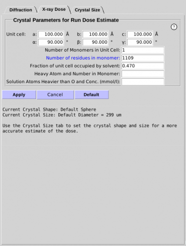
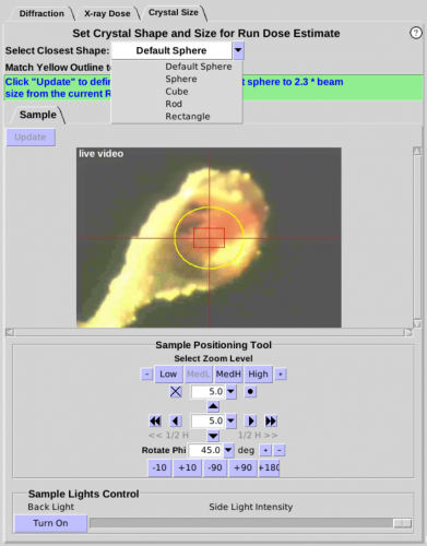
The Crystal Size sub-tab provides an interactive tool to define the shape and size of the mounted sample to give a more accurate estimate of the absorbed dose (Fig. 7). A yellow overlay that defines the shape and size of the crystal is displayed on the camera view of the sample. When a sample is first mounted, the shape defaults to "Default Sphere". The default state assumes the crystal is approximately the same size or larger than twice the beam size in Blu-Ice. Thus, the diameter of the Default Sphere is set to 2.3 times the current beam size in Blu-Ice (i.e. the diameter is set to the Full Width of the Gaussian beam). The Update button can be used to change the default diameter of the Default Sphere. Select a new beam size and then click on "Update" in the Crystal Size sub-tab.
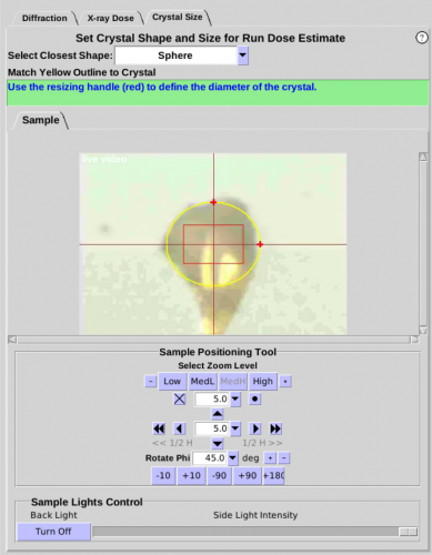
Figure 7. The Crystal Size sub-tab is used to define the shape and size of the crystal using a graphical interface. The Default Sphere shape assumes the crystal is larger than twice the beam size in Blu-Ice.(full width of the Gaussian beam). (click to enlarge). Additional shapes with handles are available in the drop down menu to better match the crystal shape and size for a more accurate Dose Estimate (Fig. 8). Choose the shape that most closely resembles the shape of the crystal. Resizing handles will appear on the yellow overlay for Sphere and Rod (Fig.9). If the beamline provides two camera views, either view can be used to adjust the size of the overlay. Grab and move the handles with the mouse (click and hold) to adjust the size of the circle/box to best fit the crystal. Handles that are colored the same adjust the shape in the same way. The crystal should be rotated about the Phi axis to verify the crystal shape and size are adequately defined.
Figure 8. The nominal shape of the crystal can be selected from the drop down menu (click to enlarge).
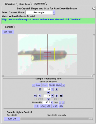
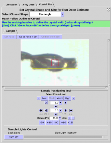
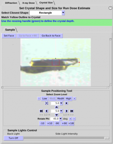
Figure 9. Sphere and Rod shapes display handles on the yellow overlay to match the crystal size (click to enlarge). Note: The Predicted Dose is immediately updated whenever the shape is changed or when the handles are used to change the size of the crystal. When Cube or Rectangle are selected (Fig. 10), the crystal should be rotated about the Phi axis to align one of the faces of the crystal approximately normal to the camera view. Once the face of the crystal is aligned, click on "Set Face" and two handles will appear for adjusting the size of the yellow overlay to match the face of the crystal (Fig. 11). Use the "Face +90" button to verify the yellow outline aligns with the crystal as it is rotated. For the Rectangle shape, an additional handle (green) will be available at the Face +90 position. Use the green handle to define the 3rd dimension of a rectangular crystal (Fig. 12).
Figure 10. When Rectangle or Cube is selected, the crystal needs to be rotated to a face before clicking on "Set Face" (Click to enlarge).
Figure 11. Once a "Face" on the crystal is "Set" for Rectangle or Cube, the yellow outline can be adjusted to the face using handles (Click to enlarge).
Figure 12. Clicking on the "Face +90" button rotates the sample exactly 90 degrees. For a Rectangle shape, a green handle will appear at this position which can be used to define the crystal length in the 3rd dimension. (Click to Enlarge) To use a different orientation of the crystal as the initial "Face" of the Cube or Rectangle, rotate Phi to the new location and click on the "Reset Face" button. The Cube or Rectangle overlay can now be resized at this new Phi position. Note: If the crystal is not clearly visible, the crystal can be rastered using low-dose x-rays to provide a reasonable estimate of the crystal size. See the Rastering Tab for more information on how to raster the crystal.
Diffraction Quality Strip Chart
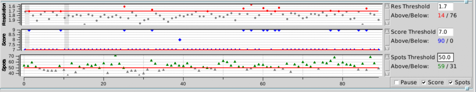
The strip chart at the bottom of the Collect Tab displays a few key data processing statistics in near real time (Fig. 15). The program Interceptor is used to quickly process each image as it is produced and the results are displayed in the strip chart. Resolution, a Quality Score and the Number of Spots are determined for each image. The Score is primarily based on resolution, with penalties and bonuses applied for number of ice rings, max intensity between 15-4.5Å, and spot elongation. Thresholds can be set to indicate the number of images/frames that meet a particular threshold (in color) and those that do not (in black). The chart can be paused by checking the Pause checkbox. The Score and Spots charts can be toggled on or off by selecting the respective checkbox. The window can be resized vertically by clicking on and dragging the square in the upper right corner of the window. Warning: These on-the-fly calculated statistics are not as accurate as fully processed data. For a more accurate assessment of your sample, please check the Automated Processing directories for your particular dataset.
Figure 15. The Diffraction Quality Strip Chart in the Collect Tab displays processing statistics in near real time. Hovering over the chart area will produce a cross cursor which can be used to select an area to zoom into (click and drag). Multiple zooms can be used to see individual data points when collecting images rapidly. Use Zoom Out in the context menu (right click on the chart area) to zoom out to the previous zoom area . Select View All to see all the data on the chart. Hovering over a data point will bring up its value and image number. Clicking on a data point will display the associated diffraction image in the Diffraction Sub-Tab. To resume displaying images as data is collected, uncheck the Hold Image checkbox in the Diffraction Tab (see Fig 14).
Automated Data Processing
Once a Run has completed, the data is automatically processed providing quick feedback on the quality of the dataset. The following directory contains the processing results: /data/account_name/data_collection_directory/auto-processing-file_name Auto-indexing and integration are carried out with LABELIT and XDS. The data are analyzed with POINTLESS and XTRIAGE, scaled and merged with AIMLESS, and transformed to amplitudes with TRUNCATE. A free R-set is also generated using 5% of the reflections. All programs use default settings with no resolution or I/sig(I) cutoffs. The input files can be modified and each step can be rerun using the run.csh scripts located in each program subdirectory,
Helical Data Collection
Overview
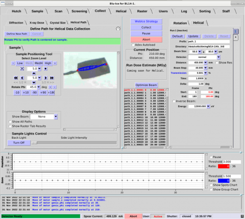
The Helical Tab is located on the Collect Tab, next to the standard Rotation Tab (Fig. 16). The accompanying Helical Path Sub-Tab is located next to the Crystal Size Tab. These tabs allow collection of oscillation data while the sample is translated along a predefined Path. On BL7-1, BL14-1 and BL9-2, the software collects an oscillation image then translates the sample to a new position and collects the next image, etc, On BL12-1 and BL12-2, the software collects oscillation data in a continuous shutterless mode by setting the speed of the translation for a constant exposure time.
Figure 16. New Helical Tab and Helical Path Sub-Tab for helical data collection. The helical Path is defined in the new Helical Path Sub-Tab. (Click to Enlarge). Since the best strategy to minimize radiation damage is to collect from the largest possible volume of the crystal, use Helical Data Collection when the beam can be spread over the volume of the sample. When possible, maximize the vertical beam size to match the vertical size of the sample and translate along the phi axis (horizontal). The Path is defined by creating a graphic overlay on the live video stream of the sample in the new Helical Path Sub-Tab (described in detail below). Helical data collection is initiated and managed in the same way as standard Rotation data collection which is described extensively above in the Collect Tab Manual.
Helical Tab
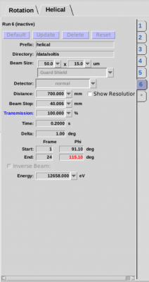
The Helical Tab (Fig. 17) is similar to the standard Rotation Tab (however, there is no "0" Tab). Helical Paths must be defined for each Run in the Helical Path Sub-Tab. Up to 16 Runs with different individual Paths on the same crystal (or multiple crystals on a mesh) can be created by clicking on the "*" Tab. Similar to the Rotation Tab (section Data Collection Parameters and Commands), the Prefix and Directory name for the images can be specified. Data collection parameters such as Beam Size, Detector Distance, Beam Stop Distance, Attenuation, Rotation Angle Delta, Exposure Time and Energy can also be set for each Run/Path.
Figure 17. The Helical Tab. Setup data collection parameters for helical data collection. Any number of Frames can be specified. For BL12-1 and BL12-2 where shutterless data collection is employed, the speed is adjusted for an even exposure of the sample as it is translated and rotation images are collected. The Default Button will set a default number of Frames for the existing Path so that the exposure overlap is ~1/2 the horizontal Gaussian beam size. If a larger dataset is desired, the number of frames can be increased with a commensurate increase in the overlap of the exposure area (typical strategy for collecting a full data set from a single crystal). Likewise, exposures can be set farther apart at the expense of collecting less Frames.
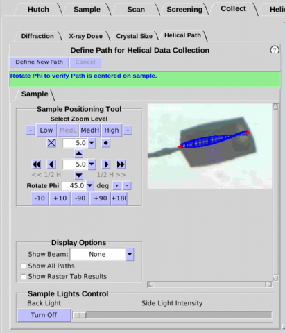
Helical Path Sub-Tab
The Helical Path Sub-Tab provides a graphical overlay on the live camera view of the sample to set a Path for helical data collection (Fig. 18). One Path can be defined for each Run and up to 16 Runs (and thus 16 Paths) can be specified for each mounted crystal (or multiple crystals on a mesh). Choose one end of your sample for the starting point of the helical Path. Align the starting point in the center of the beam (at phi and phi +90). Press "Save Path Start". Choose the end of the helical path and center it at the beam center. Press "Save Path End". Note: it is critical to rotate Phi 360 degrees to verify the positioning of the Path is correct on the sample. Note: the graphical overlay is a projection for each exposure; the horizontal beam size stays constant while the vertical beam (projected at different Phi rotation values) changes in size.
Figure 18. The Helical Path Sub-Tab for defining a helical Path using a video overlay. To modify the Path, press "Define New Path". By default, only the associated Path is shown for the selected Run as an overlay on the sample camera video. All Paths can be shown by clicking on the "Show All Paths" checkbox. In addition, results from the Raster Tab can be overlaid on the sample by selecting the Show Raster Tab Results checkbox. |